Chi-squared tests
NRES 710
Fall 2022
Download the R code for this lecture!
To follow along with the R-based lessons and demos, right (or command) click on this link and save the script to your working directory
Overview: Chi-squared-tests
Assumptions of Chi-squared tests
- Response variable (and predictor variable, for test for
independence) must be categorical (data can be summarized as
contingency table)
- Samples must be independent (this is almost always an assumption of
our classical statistical tests)
- Samples must be representative of the population of interest (again,
this is always a key assumption)
- There must be a sufficient sample size such that the expected number of observations in each element of the contingency table is at least 5!
The Chi-squared statistic:
\(\chi^2 = \sum_{i=1}^k\frac{(x_i-exp_i)^2}{exp_i}\)
Here, \(exp_i\) is the expected number of observations (count) in category i (e.g., under the null hypothesis). \(x_i\) is the observed number/count in category i. So the Chi-squared statistic basically summarizes the degree to which the observed count disagrees with the expected count across all categories.
Why is the numerator squared? First, this makes all deviations positive- negatives and positives can’t cancel each other out. Second, it allows us to use the well-described Chi-squared distribution!
The Chi-squared distribution
The Chi-squared distribution is described (like the t distribution) by a certain degrees of freedom (‘degrees of freedom’ is the parameter needed to describe the distribution – just like mean and standard deviation are parameters of the normal distribution).
If you are performing a goodness-of-fit test, the degrees of freedom for this test is one less than the number of categories.
If you are performing a test for independence of two categorical variables, the degrees of freedom is computed as \((r-1)(c-1)\) where r and c are the number of categories in each of the two categorical variables, respectively.
Chi-square goodness-of-fit test.
This test asks the question “do the observations sort into categories according to your (null) hypothesis?” In a Chi-square goodness-of-fit test, the response variable of interest is categorical. Like the one-sample t-test, there is no predictor variable.
Example: Are graduate students more likely to be born some months versus other months?
What is the population? sample? parameter? statistic?
In this example, the response variable of interest is the birth month- which is best considered a categorical variable. You can run this test on non-categorical variables (e.g., continuous numeric), but you have to turn your variable into a categorical variable (e.g., by “binning”) prior to conducting this analysis.
Example in R
## Chi squared goodness-of-fit example

birthdays.bymonth <- c(40,23,33,39,28,29,45,31,22,34,44,20)
months <- c("Jan","Feb","Mar","Apr","May","Jun","Jul","Aug","Sep","Oct","Nov","Dec")
names(birthdays.bymonth) <- months

sample.size <- sum(birthdays.bymonth)
k = length(birthdays.bymonth)   # number of categories (months)
exp.birthdays.bymonth <- sample.size*rep(1/k,times=k)   # compute the expected number under the null hypothesis.

Chisq.stat <- sum((birthdays.bymonth-exp.birthdays.bymonth)^2/exp.birthdays.bymonth)
Chisq.stat
## [1] 24.14433## View the summary statistic along with its sampling distribution under the null hypothesis
curve(dchisq(x,k-1),0,75)
abline(v=Chisq.stat,col="green",lwd=3)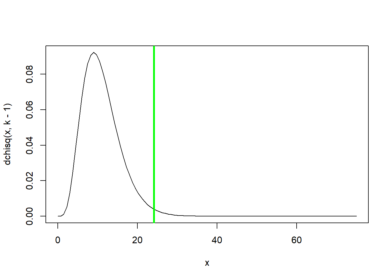
p <- 1-pchisq(Chisq.stat,k-1)
p
## [1] 0.01213825### use R's built in chi squared function
chisq.test(birthdays.bymonth) # should get the same p value!##
## Chi-squared test for given probabilities
##
## data: birthdays.bymonth
## X-squared = 24.144, df = 11, p-value = 0.01214Here is another example- this time we use a Chi-squared goodness of fit test to assess normality of a continuous variable. This example is meant to enhance understanding of the chi-squared goodness of fit test– I don’t suggest running this test to assess normality, since the shipiro-wilks test is a better test!
# Chi-squared test for normality

normal.data <- rnorm(250,4,1.5)  # generate normal data
nonnormal.data <-  runif(250,2,6)  # generate non-normal data

hist(normal.data)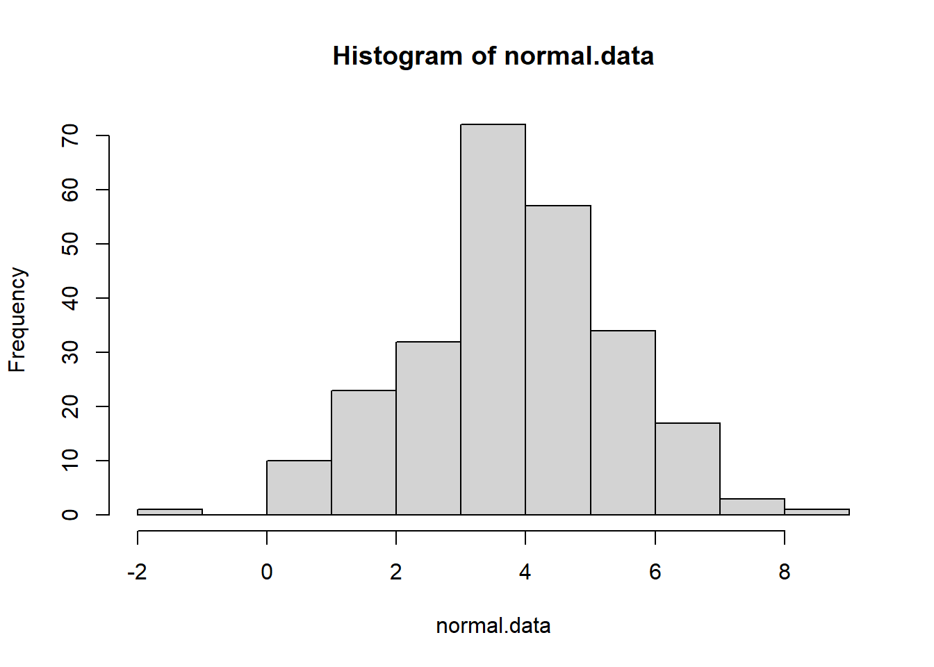
hist(nonnormal.data)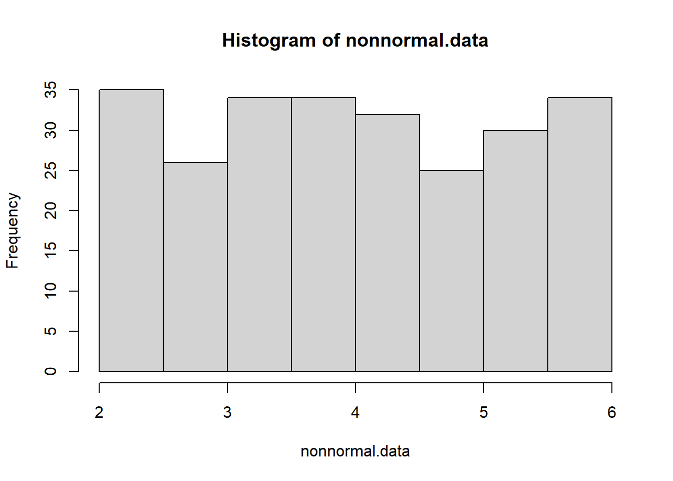
# First bin the data (chi squared test must be on categorical data!)

breaks <- c(-Inf,1,2,3,3.5,4,4.5,5,6,7,Inf)

normal.data.binned <- cut(normal.data,breaks,labels=breaks[-1])
nonnormal.data.binned <- cut(nonnormal.data,breaks,labels=breaks[-1])

obs_table_norm <- table(normal.data.binned)
obs_table_nonnorm <- table(nonnormal.data.binned)

# Determine expected values in each cell if the underlying distribution were normal

normal.probs <- sapply(2:length(breaks), function(t) pnorm(breaks[t],mean(normal.data),sd(normal.data))-pnorm(breaks[t-1],mean(normal.data),sd(normal.data))  )
exp_table_norm <- length(normal.data)*normal.probs  # check that expected vals are greater than 5

normal.probs <- sapply(2:length(breaks), function(t) pnorm(breaks[t],mean(nonnormal.data),sd(nonnormal.data))-pnorm(breaks[t-1],mean(nonnormal.data),sd(nonnormal.data))  )
exp_table_nonnorm <- length(normal.data)*normal.probs  # check that expected vals are greater than 5

# Chi squared stat for normality test on normal data

chistat_norm <- sum((obs_table_norm-exp_table_norm)^2/exp_table_norm)
pval_norm <- 1-pchisq(chistat_norm,length(exp_table_norm)-1)
pval_norm
## [1] 0.1633256chistat_nonnorm <- sum((obs_table_nonnorm-exp_table_nonnorm)^2/exp_table_nonnorm)
pval_nonnorm <- 1-pchisq(chistat_nonnorm,length(exp_table_nonnorm)-1)
pval_nonnorm## [1] 1.785932e-09# Compare with shapiro wilk test (which is a MUCH better test!)
shapiro.test(normal.data)##
## Shapiro-Wilk normality test
##
## data: normal.data
## W = 0.9955, p-value = 0.6817shapiro.test(nonnormal.data)##
## Shapiro-Wilk normality test
##
## data: nonnormal.data
## W = 0.94983, p-value = 1.392e-07Chi-square test for independence
In the chi-square test for independence, we are testing for a relationship between two categorical variables. That is, both your response variable and predictor variables are categorical. For example, we might test if rabbit ear type (floppy, pointy, mixed) is associated with rabbit coat color (white, brown, mixed) (e.g., are floppy eared rabbits more likely to be white than bunnies with pointy ears).
Example in R
Here we are testing if bunnies ear type is related to coat color. First we summarize the number of bunnies with each possible combination of coat color and ear type (this is our contingency table). Then we determine what number would be expected in each category if the null hypothesis were true. Finally we can compute the chi-squared statistic and compare with the null sampling distribution (chi squared distribution). Here is the code:
n.bunnies <- 112

    # sample assuming null hypothesis is true
all.bunnies <- data.frame(
  ear_type = sample(c("floppy","pointy","mixed"),n.bunnies,replace = T),
  coat_color = sample(c("white","brown","mixed"),n.bunnies,replace = T)
)

head(all.bunnies)
## ear_type coat_color
## 1 floppy mixed
## 2 pointy brown
## 3 pointy brown
## 4 pointy mixed
## 5 pointy brown
## 6 floppy mixed# make contingency table
con_table <- table(all.bunnies$ear_type,all.bunnies$coat_color)
# generate expected values
prop.ears <- rowSums(con_table)/n.bunnies
sum.coats <- colSums(con_table)
exp_table <- sapply(1:ncol(con_table),function(t) sum.coats[t]*prop.ears)
colnames(exp_table) <- colnames(con_table)
# compute chi-squared statistic
Chisq.stat <- sum((con_table-exp_table)^2/exp_table)
# Compare chi squared statistic with null sampling distribution
curve(dchisq(x,4),0,10)
abline(v=Chisq.stat,col="blue",lwd=2)
p.value <- 1-pchisq(Chisq.stat,4)
p.value## [1] 0.08196423text(7,0.15,paste0("p = ",round(p.value,3)))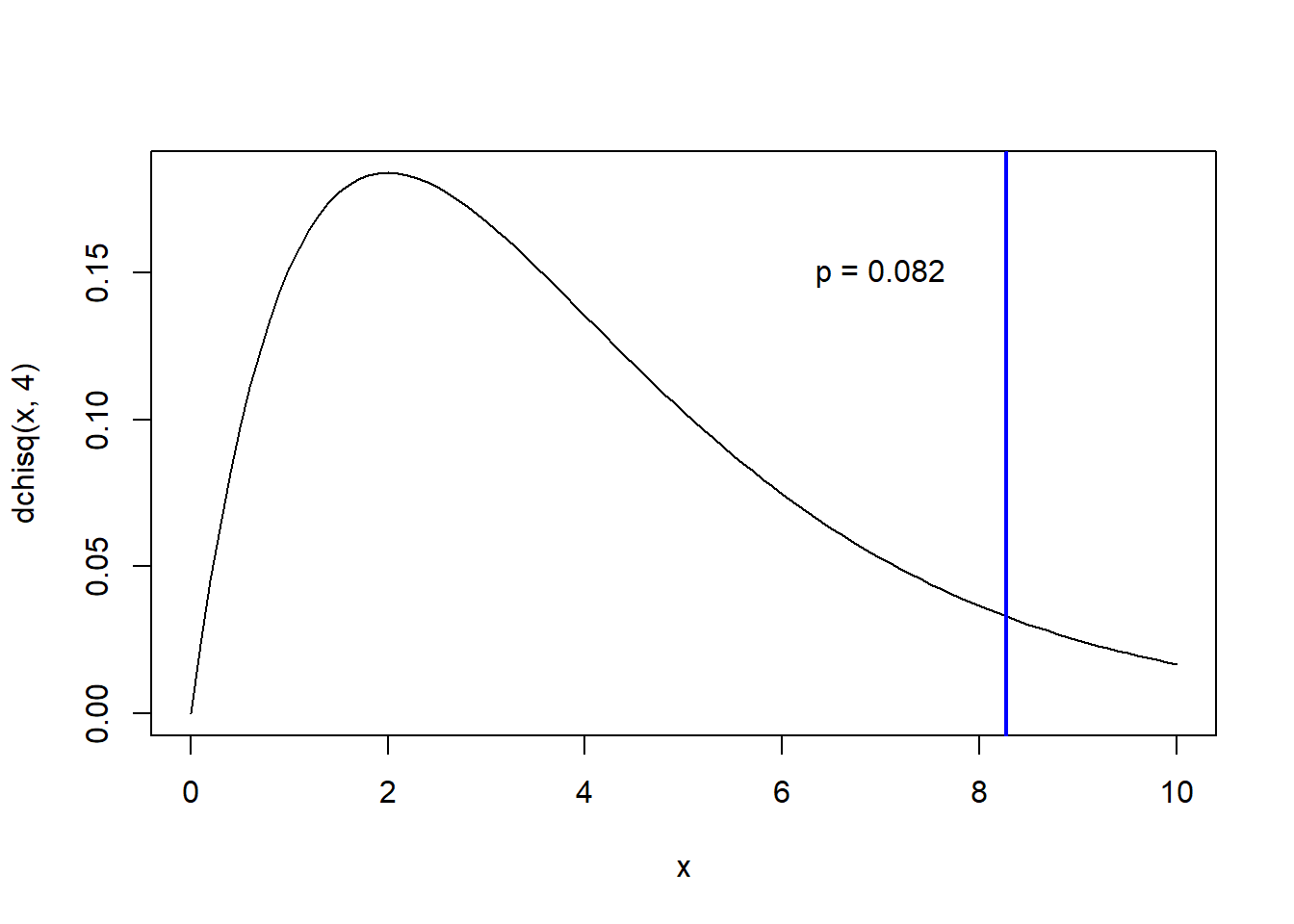
# Compare with R's built in chi squared function

chisq.test(con_table)
##
## Pearson's Chi-squared test
##
## data: con_table
## X-squared = 8.2763, df = 4, p-value = 0.08196G test
Many statistical tests recommend the G test as an alternative to the Pearson Chi-squared test. The test is very similar to the Chi Squared test, and has the same number of degrees of freedom. The G statistic is computed as:
\(G = 2\cdot \sum{O_i\cdot ln(\frac{O_i}{E_i})}\)
The sampling distribution for the G statistic is, for large sample sizes, approximately Chi-squared distributed with the same number of degrees of freedom as for the corresponding Chi-squared test.
Let’s repeat the bunny example above, this time using both the Chi-squared test and the G test.
n.bunnies <- 112

    # sample assuming null hypothesis is true
all.bunnies <- data.frame(
  ear_type = sample(c("floppy","pointy","mixed"),n.bunnies,replace = T),
  coat_color = sample(c("white","brown","mixed"),n.bunnies,replace = T)
)

head(all.bunnies)
## ear_type coat_color
## 1 mixed mixed
## 2 mixed brown
## 3 mixed white
## 4 mixed white
## 5 mixed mixed
## 6 pointy white# make contingency table
con_table <- table(all.bunnies$ear_type,all.bunnies$coat_color)
# generate expected values
prop.ears <- rowSums(con_table)/n.bunnies
sum.coats <- colSums(con_table)
exp_table <- sapply(1:ncol(con_table),function(t) sum.coats[t]*prop.ears)
colnames(exp_table) <- colnames(con_table)
# compute chi-squared and G statistics
Chisq.stat <- sum((con_table-exp_table)^2/exp_table)
G.stat <- 2*sum(con_table*log(con_table/exp_table)) # slightly different!
# Compare chi squared and G statistics with null sampling distribution
curve(dchisq(x,4),0,10)
abline(v=Chisq.stat,col="blue",lwd=1)
abline(v=G.stat,col="red",lwd=1)
legend("topright",lty=c(1,1),lwd=c(1,1),col=c("blue","red"),legend=c("Chi-squared","G stat"),bty="n")
p.value.Chi <- 1-pchisq(Chisq.stat,4)
p.value.G <- 1-pchisq(G.stat,4)
text(7,0.12,paste0("p.Chi = ",round(p.value.Chi,3)))
text(7,0.1,paste0("p.G = ",round(p.value.G,3)))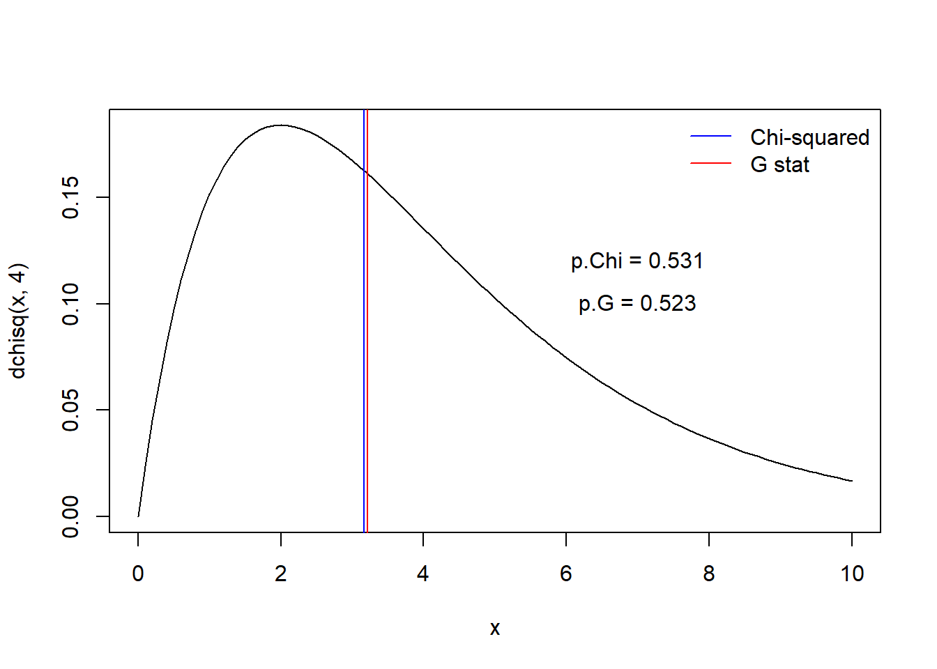
As you can see, in practice it won’t usually matter whether you use the Chi-squared or G statistic! But some reviewers may ask you to use the G statistic because most statisticians agree that it does a slightly better job than the classical Chi-squared statistic.
Non-parametric alternatives
The Chi-squared test is sometimes considered a non-parametric test because it does not assume anything about the underlying distribution of the data or the residuals. The Chi-squared tests simply makes the assumption that the observations are independent. Given the independence of observations AND large enough sample size, the sampling distribution for the chi-squared statistic (and G statistic) should be distributed according to a chi-squared distribution with the appropriate degrees of freedom.
BUT… the Fisher exact test makes fewer assumptions than the Chi-squared test– namely that the sample size is ‘large enough’ and should be used in place of the Chi-squared test when you have small sample size. Here is the bunny example again, this time with small sample size:
n.bunnies <- 20

    # sample assuming null hypothesis is true
all.bunnies <- data.frame(
  ear_type = sample(c("floppy","pointy","mixed"),n.bunnies,replace = T),
  coat_color = sample(c("white","brown","mixed"),n.bunnies,replace = T)
)

head(all.bunnies)
## ear_type coat_color
## 1 pointy mixed
## 2 pointy brown
## 3 floppy brown
## 4 pointy brown
## 5 mixed mixed
## 6 pointy white# make contingency table
con_table <- table(all.bunnies$ear_type,all.bunnies$coat_color)
# generate expected values
prop.ears <- rowSums(con_table)/n.bunnies
sum.coats <- colSums(con_table)
exp_table <- sapply(1:ncol(con_table),function(t) sum.coats[t]*prop.ears)
colnames(exp_table) <- colnames(con_table)
# run fisher exact test
#?fisher.test
chisq.test(con_table)##
## Pearson's Chi-squared test
##
## data: con_table
## X-squared = 4.3333, df = 4, p-value = 0.3628fisher.test(con_table) # better test##
## Fisher's Exact Test for Count Data
##
## data: con_table
## p-value = 0.4312
## alternative hypothesis: two.sidedfisher.test(con_table,simulate.p.value = T,B=5000) # use simulated p-value - usually very similar answer##
## Fisher's Exact Test for Count Data with simulated p-value (based on
## 5000 replicates)
##
## data: con_table
## p-value = 0.4323
## alternative hypothesis: two.sided