ANOVA
NRES 710
Fall 2022
Download the R code for this lecture!
To follow along with the R-based lessons and demos, right (or command) click on this link and save the script to your working directory
Overview: ANOVA
ANOVA is short for “ANalysis Of VAriance”. An ANOVA test is designed to assess whether the mean value is the same across groups defined by one or more categorical predictor variables. Which is another way of saying that ANOVA is a regression model where the predictor variable(s) is categorical!
In a simple linear regression, we are testing whether the mean of our response variable changes linearly across the range of our (continuous/numeric) predictor variable.
In ANOVA, we are testing whether the mean of our response variable changes across the different levels (bins) of our categorical variable.
The null hypothesis in ANOVA is that the mean of the response variable is the same across all levels of your categorical variable – i.e. \(\mu_1=\mu_2=\mu_3=\mu_i\). In this way, ANOVA is a global test that considers all of the categories of your predictor variable simultaneously. If you reject the null hypothesis, at least one of the categories is different from the others… But you don’t know which one(s)!
Note that if you’re facing a situation where your categorical variable has two groups, you can use EITHER a t-test or an ANOVA. …But you should use the t-test – first, the t-test works with unequal variance, second, there is no on-tailed F test, and third, it would just seem strangely overcomplicated to run an ANOVA in this case!
In ANOVA, the test statistic is called the F-statistic. This is analogous to the t-statistic and the Chi-squared statistic in that it has a known sampling error distribution.
Let’s explore this statistic in a little more detail!
The F Statistic
Remember that the t statistic is essentially a signal to noise ratio: you take the signal (difference between the sample mean and the null mean) and divide it by the noise (standard error of the mean).
The F-statistic is also a signal to noise ratio. The F statistic represents the signal (differences among the group means; explained variance) divided by the noise (within-group variability; unexplained variance).
Specifically, the F statistic is defined as:
\(F = \frac{between-group \space variability}{within-group \space variability}\)
The explained variance is defined by:
\(\sum_{i=1}^{K}n_i\cdot (\bar{Y_i}-\bar{Y})^2/(K-1)\)
Where K is the number of groups, \(n_i\) is the number of observations in the ith group, \(\bar{Y_i}\) is the sample mean in the ith group, and \(\bar{Y}\) is the overall mean.
The unexplained variance is defined by:
\(\sum_{i=1}^{K}\sum_{j=1}^{n_i}(Y_{ij}-\bar{Y_i})^2/(N-K)\)
You won’t generally need to compute the F-statistic yourself but it is useful to know how to do it! We will go though one example where we compute the F statistic ‘by hand’ (in R), but after that we will let R functions do the job for us!
The F Distribution
The F distribution was developed by George Snedecor (founder of the first US statistics department – at Iowa State. The “F” is in honor of Ronald Fisher, who developed the ANOVA testing framework.
Just like the t distribution and the Chi-squared distribution, the F distribution is the approximate sampling distribution of the F statistic.
Interesting fact: in the case where the categorical variable has only two levels, the F distribution is the square of the t distribution!
The F distribution has two parameters: the numerator degrees of freedom (df1; also known as the ‘treatment’ degrees of freedom) and the denominator degrees of freedom (df2; also known as the residual degrees of freedom). The numerator degrees of freedom for a one-way ANOVA is K-1, and the denominator degrees of freedom is N-K.
Regression and the F distribution/statistic
What is the F-distribution commonly associated with (besides ANOVA)? That’s right – Linear Regression!
ANOVA is a special case of regression where the predictor variable is categorical – there is one independent variable and one or more dependent variables that are categorical.
In linear regression, just as in ANOVA, the F-test is a global test of whether the signal outweighs the noise beyond a reasonable doubt!
Assumptions of ANOVA
Since ANOVA and regression are basically the same thing, the assumptions are also basically the same!
Also note that, like regression and t-tests, ANOVA is reasonably robust against violations of normality.
Normality
Each sample group is drawn from a normally distributed population. (remember the raw distribution of your response variable does not need to be normally distributed)
Independence
Samples are independent of each other (as always!)
Equal variance
All sample groups have the same variance. Note that this is equivalent to the homoskedasticity assumption from linear regression!
NOTE: you don’t really need to worry so much about ‘high influence’ points in ANOVA (although you do need to worry about outliers!). However, ANOVA works best if there are similar numbers of observations in each group - this is a ‘balanced’ design.
Examples
One-way ANOVA ‘by hand’
Let’s look at the following example: we measure the height of some plants under the effect of 3 different fertilizer treatments.
Here the individual observations (\(y_{ij}\)) are a function of the average height of the plants (\(\mu\)) plus the effect of the fertilizer (Ai) plus an error term (Eij)
To illustrate the similarity with linear regression (using the ‘language’ of linear regression), let’s write out this model as a linear equation!
\(height_i = \beta_0 + \beta_1\cdot fertilizer2 + \beta_2\cdot fertilizer3 + \epsilon_i\)
Where i is the observation number, beta0 is the intercept, beta1 and beta2 are ‘regression’ coefficients, and fertilizer2 and fertilizer3 are dummy variables or indicator variables that take the value 0 or 1. For example, if observation 11 was treated with fertilizer #2, then the value for ‘fertilizer2’ would be 1 and the value for ‘fertilizer3’ would be zero.
What happened to fertilizer #1 in this example? Well, if observation 5 was treated with fertilizer #1, then the value for ‘fertilizer2’ would be 0 and the value for ‘fertilizer3’ would also be zero. That is, the intercept (beta0) represents the expected mean for observations treated with fertilizer 1!
[demonstration with ‘model.matrix’]
Our goal here is to test if the regression coefficients beta1 and beta2 are zero- that is, that mean plant height is the same across all three treatments (in regression terms: the intercept-only model is the correct model).
# Simple one-way ANOVA example---------------

F1 <- c(1,2,2,3)     # plant height under fertilizer treatment 1
F2 <- c(5,6,5,4)
F3 <- c(2,1,2,2)

# combine into single dataframe for easier visualization and analysis

df <- data.frame(
  Height = c(F1,F2,F3),
  Treatment = rep(c("F1","F2","F3"),each=length(F1)),
  stringsAsFactors = T
)

plot(Height~Treatment, data=df)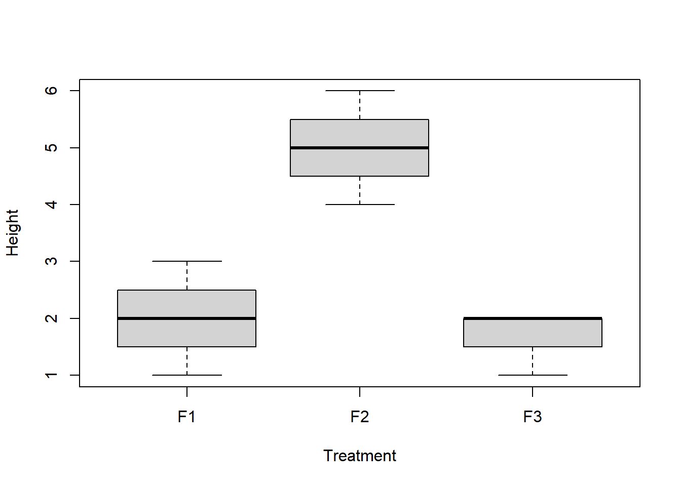
Our goal is to assess the incompatibility of the data with the null hypothesis that the group means are equal.
grand.mean <- mean(df$Height)   # grand mean

group.means <- by(df$Height,df$Treatment,mean)    # group means

n.groups <- length(group.means)   # number of groups

group.sample.size <- by(df$Height,df$Treatment,length)

sample.size <- nrow(df)

explained.var <- sum(group.sample.size*(group.means-grand.mean)^2/(n.groups-1))

groups <- lapply(1:n.groups,function(t) df$Height[df$Treatment==levels(df$Treatment)[t]])

residual.var <- sapply(1:n.groups,function(t) (groups[[t]]-group.means[t])^2/(sample.size-n.groups) )

unexplained.var <- sum(residual.var)

###
# now we can compute the F statistic!

Fstat <- explained.var/unexplained.var
Fstat
## [1] 24.78947###
# define degrees of freedom
df1 <- n.groups-1
df2 <- sample.size-n.groups
###
# visualize the sampling distribution under null hypothesis
curve(df(x,df1,df2),0,10)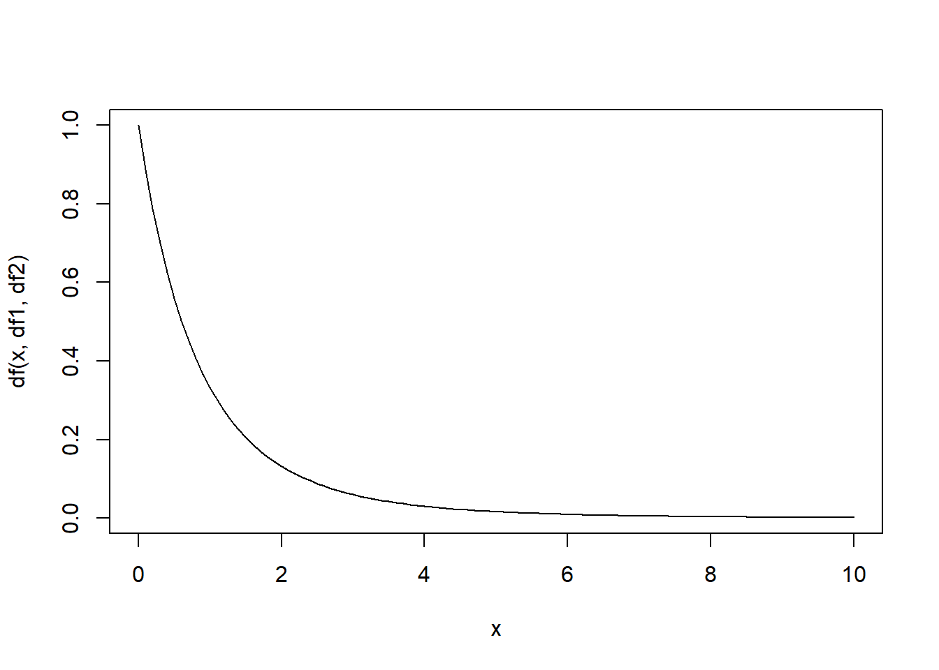
###
# compute critical value of F statistic

Fcrit <- qf(0.95,df1,df2)
Fcrit
## [1] 4.256495###
# compute p-value
pval <- 1-pf(Fstat,df1,df2)
###
# use aov function
model1 <- aov(Height~Treatment,data=df)
summary(model1)## Df Sum Sq Mean Sq F value Pr(>F)
## Treatment 2 26.17 13.083 24.79 0.000218 ***
## Residuals 9 4.75 0.528
## ---
## Signif. codes: 0 '***' 0.001 '**' 0.01 '*' 0.05 '.' 0.1 ' ' 1###
# use lm function
model.matrix(Height~Treatment,data=df)## (Intercept) TreatmentF2 TreatmentF3
## 1 1 0 0
## 2 1 0 0
## 3 1 0 0
## 4 1 0 0
## 5 1 1 0
## 6 1 1 0
## 7 1 1 0
## 8 1 1 0
## 9 1 0 1
## 10 1 0 1
## 11 1 0 1
## 12 1 0 1
## attr(,"assign")
## [1] 0 1 1
## attr(,"contrasts")
## attr(,"contrasts")$Treatment
## [1] "contr.treatment"model1 <- lm(Height~Treatment,data=df)
summary(model1)##
## Call:
## lm(formula = Height ~ Treatment, data = df)
##
## Residuals:
## Min 1Q Median 3Q Max
## -1.0000 -0.1875 0.0000 0.2500 1.0000
##
## Coefficients:
## Estimate Std. Error t value Pr(>|t|)
## (Intercept) 2.0000 0.3632 5.506 0.000377 ***
## TreatmentF2 3.0000 0.5137 5.840 0.000247 ***
## TreatmentF3 -0.2500 0.5137 -0.487 0.638128
## ---
## Signif. codes: 0 '***' 0.001 '**' 0.01 '*' 0.05 '.' 0.1 ' ' 1
##
## Residual standard error: 0.7265 on 9 degrees of freedom
## Multiple R-squared: 0.8464, Adjusted R-squared: 0.8122
## F-statistic: 24.79 on 2 and 9 DF, p-value: 0.0002184anova(model1)## Analysis of Variance Table
##
## Response: Height
## Df Sum Sq Mean Sq F value Pr(>F)
## Treatment 2 26.167 13.0833 24.79 0.0002184 ***
## Residuals 9 4.750 0.5278
## ---
## Signif. codes: 0 '***' 0.001 '**' 0.01 '*' 0.05 '.' 0.1 ' ' 1Pairwise comparisons
The ANOVA test is a global test, meaning that if our p-value is less than our alpha level we are able to reject the null hypothesis that all of the group means are equal to one another. But if we reject our null hypothesis we can’t say which of the group means are different.
This is where pairwise comparison comes in. Pairwise comparisons allow you to determine which pairs of means are different from one another.
Remember that if we are unable to reject our null hypothesis, there is no point in performing pairwise comparisons- we already know that the variation in group means is consistent with the null hypothesis that the true population means are not actually different from one another.
There are several ways to perform pairwise comparisons in R. One of
the most powerful and flexible functions for doing this is the
emmeans() function (in the ‘emmeans’ package).
For classical ANOVA tests, the most common method for pairwise
comparison is called ‘Tukey’s test’. This can be done using the
‘TukeyHSD’ function in R or the emmeans() function.
Tukey’s test
Tukey’s test (or Tukey’s Honestly Significant Differences [HSD]) compares all possible pairs of group means and determines if each pair is more different than could reasonably be expected under the null hypothesis.
Tukey’s test assumes that observations are normally distributed. In addition, Tukey’s test assumes independence of observations (of course!) and homogeneity of variance among groups.
The test statistic for Tukey’s test is called q, and is computed as:
\(q = \frac{Y_A-Y_B}{SE}\), where \(Y_A\) is the larger of the two means being compared.
Does this look like any other familiar test statistic? Yes, that’s right- Tukey’s test is essentially a t-test! The only difference is that it is maintaining an experimentwise error rate that matches the alpha level you set. So you could run multiple independent t-tests- one for each pair of factor levels. BUT if you did that, the more tests you ran, the higher your risk of committing a type-I error. If we use Tukey’s test, we keep that risk equal to alpha regardless of how many tests we perform.
The standard error for Tukey’s test is computed as:
\(\sqrt{(\frac{MSE}{2})(\frac{1}{n_i}+\frac{1}{n_j})}\)
With unequal sample sizes, the test is called a Tukey-Kramer test.
Tukey test example
Lets’ try it!
# Pairwise comparison! -----------------

# Tukey's test

# find critical q-value for tukey test
q.value <- qtukey(p=0.95,nmeans=n.groups,df=(sample.size-n.groups))

# find honestly significant difference
tukey.hsd <- q.value * sqrt(unexplained.var/(sample.size/n.groups))

# if differences in group means are greater than this value then we can reject the null!

## let's look at the difference between means

all_means <- tapply(df$Height,df$Treatment,mean)
all_levels <- levels(df$Treatment)
pair_totry <- matrix(c(1,2,1,3,2,3),nrow=3,byrow = T)
pair_totry     # these are the pairwise comparisons to make!
## [,1] [,2]
## [1,] 1 2
## [2,] 1 3
## [3,] 2 3thispair <- pair_totry[1,] # run first pairwise comparison
dif.between.means <- all_means[thispair[1]]-all_means[thispair[2]]
dif.between.means # since this is greater than tukey.hsd, we already know we can reject the null## F1
## -3### compute p-value!
sample.size.pergroup <- sample.size/n.groups
std.err <- sqrt(unexplained.var / 2 * (2 / sample.size.pergroup))
# first compute q statistic
q.stat <- abs(dif.between.means)/std.err
p.val <- 1-ptukey(q.stat,nmeans=n.groups,df=(sample.size-n.groups))
p.val## F1
## 0.0006459124## run all pairwise comparisons
results <- NULL
i=1
for(i in 1:nrow(pair_totry)){
thispair <- pair_totry[i,]
temp <- data.frame(
group1 = all_levels[thispair[1]],
group1 = all_levels[thispair[2]]
)
temp$dif = all_means[thispair[1]]-all_means[thispair[2]]
temp$qstat = abs(temp$dif)/std.err
temp$pval = 1-ptukey(temp$qstat,nmeans=n.groups,df=(sample.size-n.groups))
results <- rbind(results,temp)
}
results## group1 group1.1 dif qstat pval
## 1 F1 F2 -3.00 8.2589664 0.0006459124
## 2 F1 F3 0.25 0.6882472 0.8792868263
## 3 F2 F3 3.25 8.9472136 0.0003591856### compare with R's built in tukey test function
model1 <- aov(Height~Treatment,data=df)
TukeyHSD(model1)## Tukey multiple comparisons of means
## 95% family-wise confidence level
##
## Fit: aov(formula = Height ~ Treatment, data = df)
##
## $Treatment
## diff lwr upr p adj
## F2-F1 3.00 1.565743 4.434257 0.0006459
## F3-F1 -0.25 -1.684257 1.184257 0.8792868
## F3-F2 -3.25 -4.684257 -1.815743 0.0003592### and finally, compare with 'emmeans'
library(emmeans)
model1 <- lm(Height~Treatment,data=df)
emm <- emmeans(model1,specs=c("Treatment")) # compute the treatment means with 'emmeans'
pairs(emm) # run tukey test!## contrast estimate SE df t.ratio p.value
## F1 - F2 -3.00 0.514 9 -5.840 0.0006
## F1 - F3 0.25 0.514 9 0.487 0.8793
## F2 - F3 3.25 0.514 9 6.327 0.0004
##
## P value adjustment: tukey method for comparing a family of 3 estimatesNote that the last method (‘emmeans’) is the most flexible, since you can use this function for all kinds of models, including GLM!
The ‘general’ way to think about pairwise comparisons is that you are using the model to make predictions (of the mean response value) under different pairs of “what if” scenarios (e.g., what is the expected response if treatment is A vs B, given temperature is 25C, and soil type is “A”) and then testing to see if those differences are consistent with the null hypothesis of zero differences. If you think about it this way, performing pairwise comparisons can make sense even for complex models with multiple continuous and categorical predictor variables!
Another simple example
Here we run another simple example of a one-way ANOVA followed by Tukey’s pairwise comparison tests, just using R’s built in functions (no more ‘by hand’ calculations!):
library(agricolae)
data("PlantGrowth")

plant.lm <- lm(weight ~ group, data = PlantGrowth)   #run the 'regression' model
plant.av <- aov(plant.lm)  # run anova test and print anova table
plant.av
## Call:
## aov(formula = plant.lm)
##
## Terms:
## group Residuals
## Sum of Squares 3.76634 10.49209
## Deg. of Freedom 2 27
##
## Residual standard error: 0.6233746
## Estimated effects may be unbalanced###
# evaluate goodness of fit (assumption violations etc)
layout(matrix(1:4,nrow=2,byrow = T))
plot(plant.av)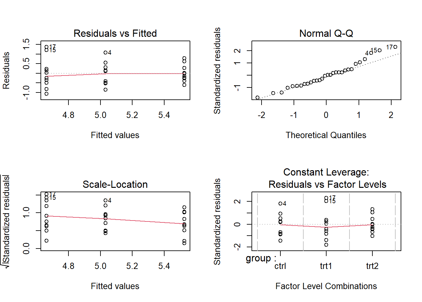
###
# run pairwise comparisons

tukeytest <- TukeyHSD(plant.av)
tukeytest
## Tukey multiple comparisons of means
## 95% family-wise confidence level
##
## Fit: aov(formula = plant.lm)
##
## $group
## diff lwr upr p adj
## trt1-ctrl -0.371 -1.0622161 0.3202161 0.3908711
## trt2-ctrl 0.494 -0.1972161 1.1852161 0.1979960
## trt2-trt1 0.865 0.1737839 1.5562161 0.0120064layout(matrix(1,nrow=1,byrow = T))
plot(tukeytest) #default plotting method for tukey test objects!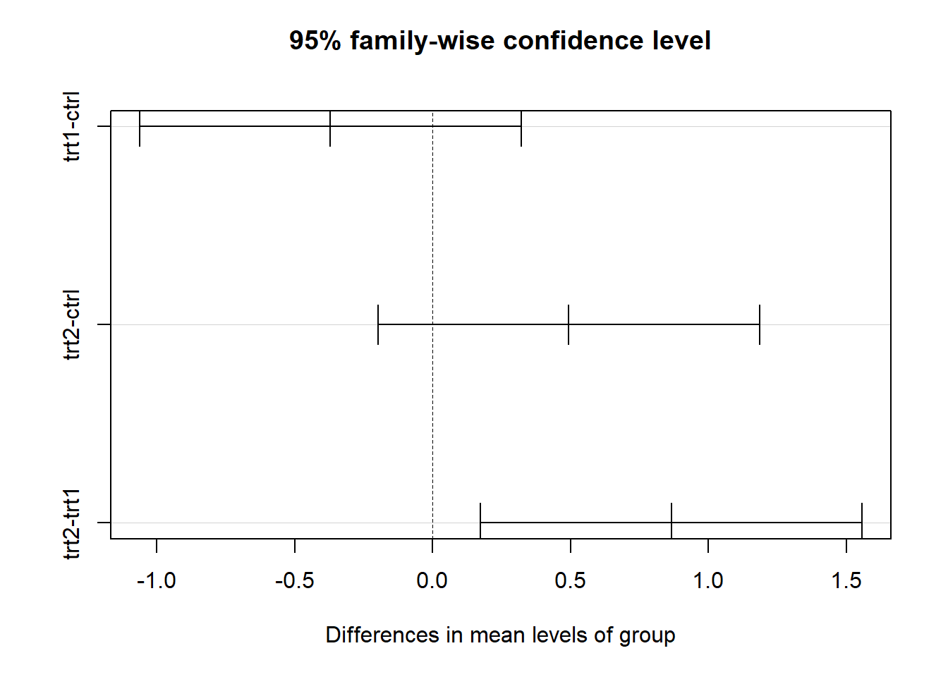
###
# alternative method

 # run tukey test
emm <- emmeans(plant.lm,specs=c("group"))  # compute the treatment means with 'emmeans'
pairs(emm)    # run tukey test!
## contrast estimate SE df t.ratio p.value
## ctrl - trt1 0.371 0.279 27 1.331 0.3909
## ctrl - trt2 -0.494 0.279 27 -1.772 0.1980
## trt1 - trt2 -0.865 0.279 27 -3.103 0.0120
##
## P value adjustment: tukey method for comparing a family of 3 estimatestoplot <- as.data.frame(summary(emm))[,c("group","emmean","lower.CL","upper.CL")]
xvals <- barplot(toplot$emmean,names.arg = toplot$group,ylim=c(0,7))
arrows(xvals,toplot$lower.CL,xvals,toplot$upper.CL,angle=90,code=3)
text(xvals,c(6.4,6.4,6.4),labels = c("ab","a","b"),cex=1.5)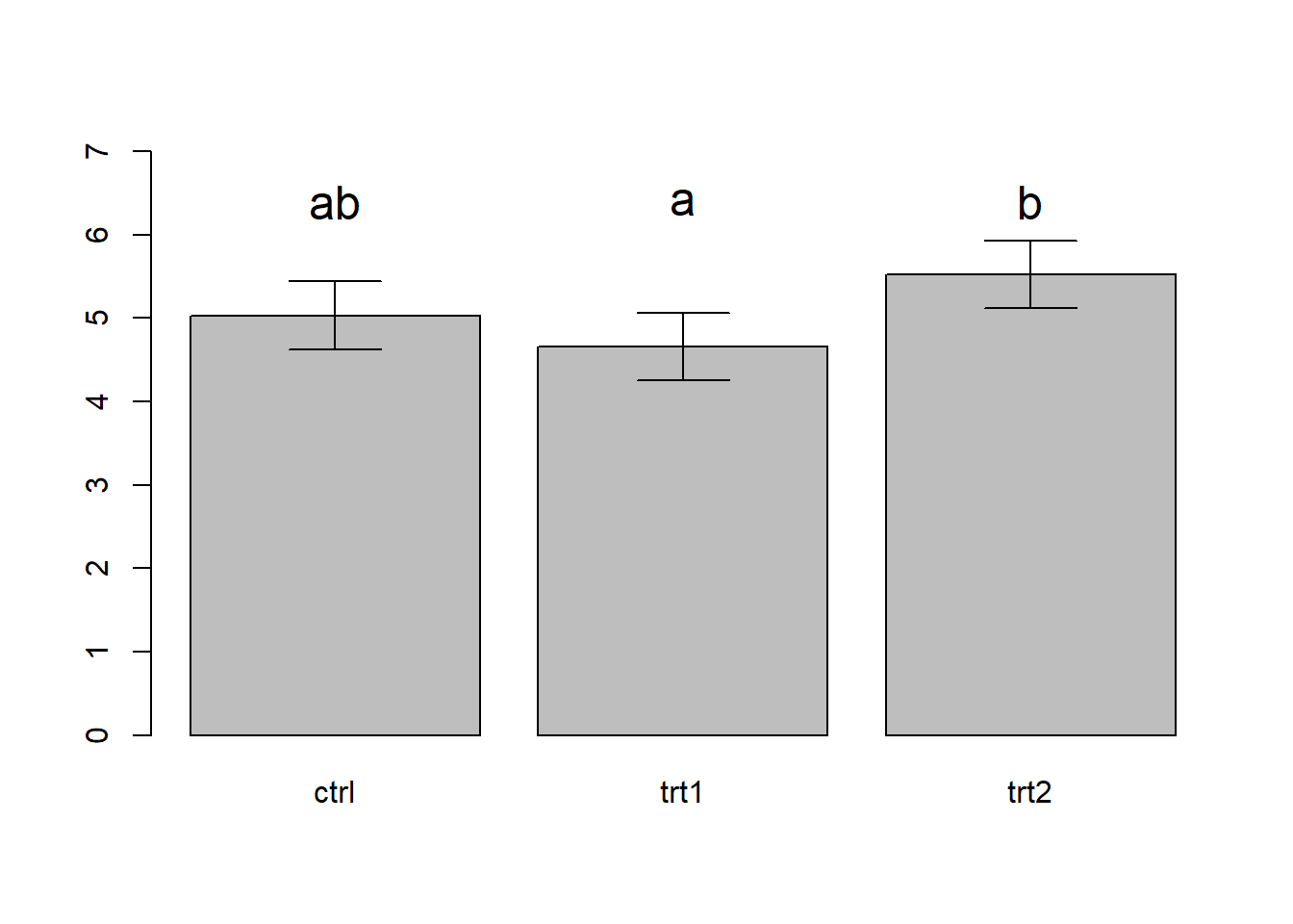
# note: many statisticians recommend against compact letter displays... In the above figure, we use the convention of adding letter codes to our plot to illustrate the results of the pairwise comparison (compact letter displays). Pairs of treatments/groups with different labels are different according to the pairwise comparison test. Pairs that share a common label are not different. In the above figure, treatment 1 and treatment 2 are different from one another, but the control is not different from either treatment. You can also see this visually based on the overlapping in the confidence intervals (trt1 and trt2 do not overlap, whereas both treatments overlap with the control).
Statisticians often warn against using compact letter displays, for the same reasons they often caution against using “significance tests” (e.g., \(p < 0.05\)).
Two-way ANOVA
When you have more than one categorical predictor variable in your ANOVA model, you are performing a multiple factor ANOVA. The simplest case is when you have two categorical variables (or factors)– this is called two-factor ANOVA (or two-way ANOVA). Multiple factor ANOVA is analogous to multi-variable linear regression.
In a two-way ANOVA, your global null hypothesis is that the mean of the response variable is not affected by either of the two factors. Secondarily, you can test the individual null hypotheses that the mean response does not vary across the levels of factor 1 or 2 separately.
Interactions
The concept of interactions is fundamental to both multiple linear regression and multiple factor ANOVA.
The basic idea is that the relationship between your response variable (e.g., fruit dry weight) and your first predictor variable (e.g., fertilizer type) varies depending on your second predictor variable (e.g., soil type). For example, maybe your plants tend to produce larger fruits when fertilized in soil type A, but do not respond to fertilization in soil type B.
In regression terminology, interaction terms look similar to any other regression coefficient. Here’s an example, continuing with the fertilizer/soil example (3 fertilization treatments, 2 soil treatments):
\(height_i = \beta_0 + \beta_1\cdot fertilizer2 + \beta_2\cdot fertilizer3 + \beta_3\cdot soil2 + \beta_4\cdot fertilizer2\times soil2 + \beta_5\cdot fertilizer3\times soil2 + \epsilon_i\)
In the above equation, \(\beta_0\) is the intercept term, \(\beta_1\) and \(\beta_2\) are the main effect terms for the “fertilizer” factor variable (same as we saw above- recall that the intercept term represents fertilizer 1) – “fertilizer2” and “fertilizer3” are dummy variables (either zero or one) indicating whether or not observations belong to these respective treatments. Similarly, the \(\beta_3\) term is the main effect of soil treatment 2 (the intercept now refers to fertilizer treatment 1, soil treatment 1).
The \(\beta_4\) and \(\beta_5\) terms are interaction coefficients. \(\beta_4\) represents the effect of fertilizer2 on plants growing in the soil2 treatment only. \(\beta_5\) represents the effect of fertilizer3 on plants growing in the soil2 treatment only. Note that the term \(fertilizer2\times soil2\) is essentially a dummy variable indicating whether or not an observation was treated with fertilizer2 AND grown in soil2. Multiplying two dummy variables together essentially results in a new, more specific dummy variable!
Interaction example
## two way interaction example

data("ToothGrowth")
summary(ToothGrowth)
## len supp dose
## Min. : 4.20 OJ:30 Min. :0.500
## 1st Qu.:13.07 VC:30 1st Qu.:0.500
## Median :19.25 Median :1.000
## Mean :18.81 Mean :1.167
## 3rd Qu.:25.27 3rd Qu.:2.000
## Max. :33.90 Max. :2.000table(ToothGrowth$supp,ToothGrowth$dose) # three doses, two types of supplements##
## 0.5 1 2
## OJ 10 10 10
## VC 10 10 10ToothGrowth$dose <- as.factor(as.character(ToothGrowth$dose)) # convert dose variable to factor (make it categorical)
model <- lm(len~supp+dose,data=ToothGrowth) # two way anova with no interaction
summary(model)##
## Call:
## lm(formula = len ~ supp + dose, data = ToothGrowth)
##
## Residuals:
## Min 1Q Median 3Q Max
## -7.085 -2.751 -0.800 2.446 9.650
##
## Coefficients:
## Estimate Std. Error t value Pr(>|t|)
## (Intercept) 12.4550 0.9883 12.603 < 2e-16 ***
## suppVC -3.7000 0.9883 -3.744 0.000429 ***
## dose1 9.1300 1.2104 7.543 4.38e-10 ***
## dose2 15.4950 1.2104 12.802 < 2e-16 ***
## ---
## Signif. codes: 0 '***' 0.001 '**' 0.01 '*' 0.05 '.' 0.1 ' ' 1
##
## Residual standard error: 3.828 on 56 degrees of freedom
## Multiple R-squared: 0.7623, Adjusted R-squared: 0.7496
## F-statistic: 59.88 on 3 and 56 DF, p-value: < 2.2e-16anova(model)## Analysis of Variance Table
##
## Response: len
## Df Sum Sq Mean Sq F value Pr(>F)
## supp 1 205.35 205.35 14.017 0.0004293 ***
## dose 2 2426.43 1213.22 82.811 < 2.2e-16 ***
## Residuals 56 820.43 14.65
## ---
## Signif. codes: 0 '***' 0.001 '**' 0.01 '*' 0.05 '.' 0.1 ' ' 1model_with_interaction <- lm(len~supp*dose,data=ToothGrowth) # now try again with interactions
summary(model_with_interaction)##
## Call:
## lm(formula = len ~ supp * dose, data = ToothGrowth)
##
## Residuals:
## Min 1Q Median 3Q Max
## -8.20 -2.72 -0.27 2.65 8.27
##
## Coefficients:
## Estimate Std. Error t value Pr(>|t|)
## (Intercept) 13.230 1.148 11.521 3.60e-16 ***
## suppVC -5.250 1.624 -3.233 0.00209 **
## dose1 9.470 1.624 5.831 3.18e-07 ***
## dose2 12.830 1.624 7.900 1.43e-10 ***
## suppVC:dose1 -0.680 2.297 -0.296 0.76831
## suppVC:dose2 5.330 2.297 2.321 0.02411 *
## ---
## Signif. codes: 0 '***' 0.001 '**' 0.01 '*' 0.05 '.' 0.1 ' ' 1
##
## Residual standard error: 3.631 on 54 degrees of freedom
## Multiple R-squared: 0.7937, Adjusted R-squared: 0.7746
## F-statistic: 41.56 on 5 and 54 DF, p-value: < 2.2e-16anova(model_with_interaction)## Analysis of Variance Table
##
## Response: len
## Df Sum Sq Mean Sq F value Pr(>F)
## supp 1 205.35 205.35 15.572 0.0002312 ***
## dose 2 2426.43 1213.22 92.000 < 2.2e-16 ***
## supp:dose 2 108.32 54.16 4.107 0.0218603 *
## Residuals 54 712.11 13.19
## ---
## Signif. codes: 0 '***' 0.001 '**' 0.01 '*' 0.05 '.' 0.1 ' ' 1NOTE: if an interaction term is ‘significant’ but the main effects terms are not significant, the standard practice is to include the main effects terms anyway! That is, it is not common practice to fit regression/ANOVA models with only interaction terms (although this is appropriate in some rare cases).
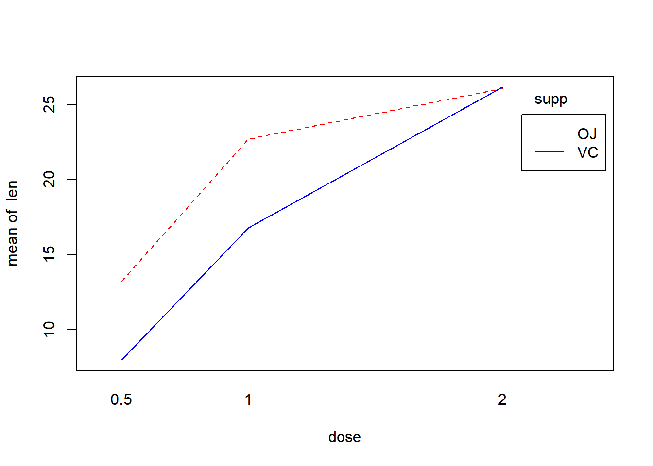
Here the results suggest that there is a significant interaction between dose and supplement type. As always, a plot can help. Let’s visualize this interaction!
# visualize the interaction

# ?interaction.plot     # this base R function can be used to visualize interactions

with(ToothGrowth, {   # the "with" function allows you to only specify the name of the data frame once, and then refer to the columns of the data frame as if they were variables in your main environment
  interaction.plot(dose, supp, len, fixed = TRUE, col = c("red","blue"), leg.bty = "o")
})
# alternatively, use the "effects" package:

plot(effects::Effect(c("dose", "supp"),model_with_interaction))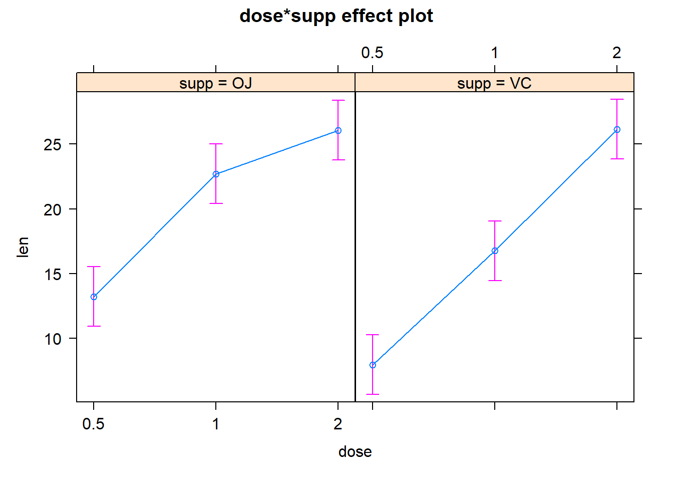
plot(effects::Effect(c("dose", "supp"),model))
Pairwise comparisons
Pairwise comparisons for two-way ANOVA are similar to in one-way ANOVA- you just have to specify which categorical predictor variable(s) you want to run pairwise comparisons for! Or, for models with interactions, you might want to run pairwise comparisons for all combinations of levels across both categorical predictors… If you want to do the latter (e.g., to examine which specific interactions are significant), you can the ‘emmeans’ package
TukeyHSD(aov(model), "dose") # run Tukey test for the 'dose' variable in the ToothGrowth model## Tukey multiple comparisons of means
## 95% family-wise confidence level
##
## Fit: aov(formula = model)
##
## $dose
## diff lwr upr p adj
## 1-0.5 9.130 6.215909 12.044091 0e+00
## 2-0.5 15.495 12.580909 18.409091 0e+00
## 2-1 6.365 3.450909 9.279091 7e-06TukeyHSD(aov(model_with_interaction), "dose") # run Tukey test for the 'dose' variable in the ToothGrowth model## Tukey multiple comparisons of means
## 95% family-wise confidence level
##
## Fit: aov(formula = model_with_interaction)
##
## $dose
## diff lwr upr p adj
## 1-0.5 9.130 6.362488 11.897512 0.0e+00
## 2-0.5 15.495 12.727488 18.262512 0.0e+00
## 2-1 6.365 3.597488 9.132512 2.7e-06library(emmeans)
emm = emmeans(model_with_interaction, ~dose:supp)
emm## dose supp emmean SE df lower.CL upper.CL
## 0.5 OJ 13.23 1.15 54 10.93 15.5
## 1 OJ 22.70 1.15 54 20.40 25.0
## 2 OJ 26.06 1.15 54 23.76 28.4
## 0.5 VC 7.98 1.15 54 5.68 10.3
## 1 VC 16.77 1.15 54 14.47 19.1
## 2 VC 26.14 1.15 54 23.84 28.4
##
## Confidence level used: 0.95plot(emm,by="dose")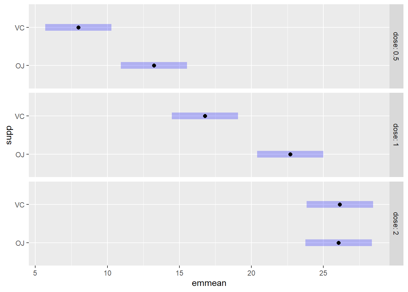
pairs(emm,type="response") # look at pairwise comparisons## contrast estimate SE df t.ratio p.value
## dose0.5 OJ - dose1 OJ -9.47 1.62 54 -5.831 <.0001
## dose0.5 OJ - dose2 OJ -12.83 1.62 54 -7.900 <.0001
## dose0.5 OJ - dose0.5 VC 5.25 1.62 54 3.233 0.0243
## dose0.5 OJ - dose1 VC -3.54 1.62 54 -2.180 0.2640
## dose0.5 OJ - dose2 VC -12.91 1.62 54 -7.949 <.0001
## dose1 OJ - dose2 OJ -3.36 1.62 54 -2.069 0.3187
## dose1 OJ - dose0.5 VC 14.72 1.62 54 9.064 <.0001
## dose1 OJ - dose1 VC 5.93 1.62 54 3.651 0.0074
## dose1 OJ - dose2 VC -3.44 1.62 54 -2.118 0.2936
## dose2 OJ - dose0.5 VC 18.08 1.62 54 11.133 <.0001
## dose2 OJ - dose1 VC 9.29 1.62 54 5.720 <.0001
## dose2 OJ - dose2 VC -0.08 1.62 54 -0.049 1.0000
## dose0.5 VC - dose1 VC -8.79 1.62 54 -5.413 <.0001
## dose0.5 VC - dose2 VC -18.16 1.62 54 -11.182 <.0001
## dose1 VC - dose2 VC -9.37 1.62 54 -5.770 <.0001
##
## P value adjustment: tukey method for comparing a family of 6 estimatespwpm(emm) # generate an informative summary matrix of pairwise comparisons!## 0.5 OJ 1 OJ 2 OJ 0.5 VC 1 VC 2 VC
## 0.5 OJ [13.23] <.0001 <.0001 0.0243 0.2640 <.0001
## 1 OJ -9.47 [22.70] 0.3187 <.0001 0.0074 0.2936
## 2 OJ -12.83 -3.36 [26.06] <.0001 <.0001 1.0000
## 0.5 VC 5.25 14.72 18.08 [ 7.98] <.0001 <.0001
## 1 VC -3.54 5.93 9.29 -8.79 [16.77] <.0001
## 2 VC -12.91 -3.44 -0.08 -18.16 -9.37 [26.14]
##
## Row and column labels: dose:supp
## Upper triangle: P values adjust = "tukey"
## Diagonal: [Estimates] (emmean)
## Lower triangle: Comparisons (estimate) earlier vs. lateremmip(model_with_interaction, supp ~ dose) # interaction plot of emms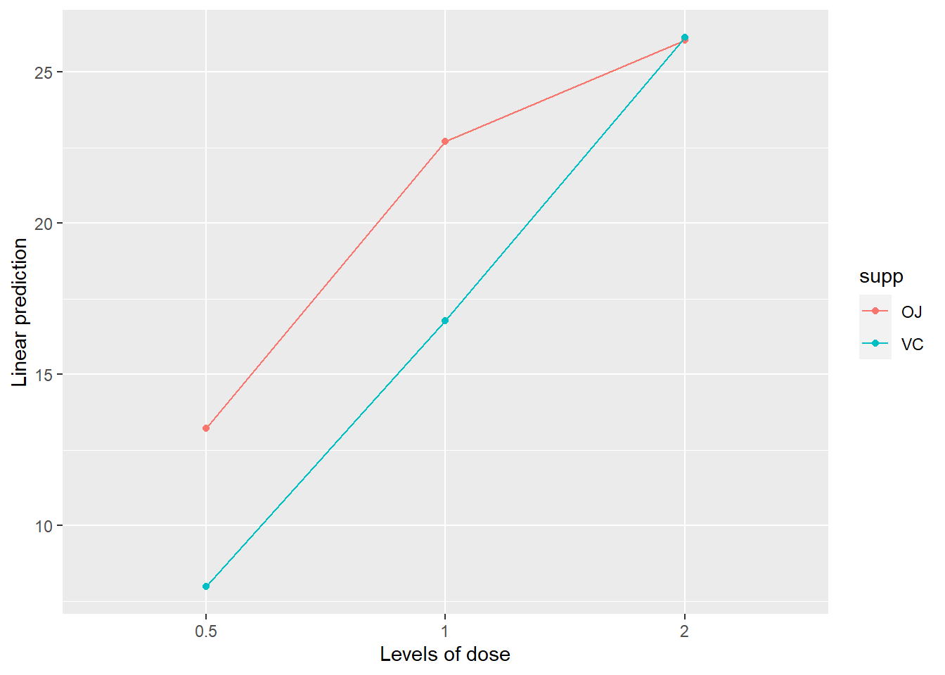
# NOTE: you could use compact letter displays but many statisticians prefer to avoid this!Non-parametric ANOVA (Kruskal-Wallis test)
If your residuals are highly non-normal and heteroskedastic (or you have severe outliers) and transformations don’t seem to help, you might want to try a non-parametric test.
The most common non-parametric version of the classical one-way ANOVA test is the Kruskal-Wallis test (K-W). Similar to a one-way ANOVA, the null hypothesis here is that all samples (regardless of group) come from the same underlying distribution. The difference is that we don’t assume that distribution is Gaussian (normally distributed)! If we reject our null hypothesis in the K-W test, we can conclude that the median value for at least one group differs from the others.
The test statistic for the K-W test is called H, and like other common non-parametric tests, it involves ranking the observations. The distribution of the H statistic is often approximated by a chi-squared distribution!
The following example comes from this site:
### Kruskal-Wallis example


## read in data:

Input =("
Group      Value
Group.1      1
Group.1      2
Group.1      3
Group.1      4
Group.1      5
Group.1      6
Group.1      7
Group.1      8
Group.1      9
Group.1     46
Group.1     47
Group.1     48
Group.1     49
Group.1     50
Group.1     51
Group.1     52
Group.1     53
Group.1    342
Group.2     10
Group.2     11
Group.2     12
Group.2     13
Group.2     14
Group.2     15
Group.2     16
Group.2     17
Group.2     18
Group.2     37
Group.2     58
Group.2     59
Group.2     60
Group.2     61
Group.2     62
Group.2     63
Group.2     64
Group.2    193
Group.3     19
Group.3     20
Group.3     21
Group.3     22
Group.3     23
Group.3     24
Group.3     25
Group.3     26
Group.3     27
Group.3     28
Group.3     65
Group.3     66
Group.3     67
Group.3     68
Group.3     69
Group.3     70
Group.3     71
Group.3     72
")

Data = read.table(textConnection(Input),header=TRUE)

Data$Group = factor(Data$Group,levels=unique(Data$Group))    # transform predictor variable to factor

#summarize values by group

groups <- unique(Data$Group)
ngroups <- length(groups)
sumry <- sapply(1:ngroups,function(i){temp <- subset(Data,Group==groups[i]); summary(temp$Value)}  )
colnames(sumry) <- groups
sumry
## Group.1 Group.2 Group.3
## Min. 1.00 10.00 19.00
## 1st Qu. 5.25 14.25 23.25
## Median 27.50 27.50 27.50
## Mean 43.50 43.50 43.50
## 3rd Qu. 49.75 60.75 67.75
## Max. 342.00 193.00 72.00# histograms by group
library(ggplot2)
ggplot(Data, aes(x=Value)) +
geom_histogram(bins=10,aes(color=Group,fill=Group)) +
facet_grid(~Group)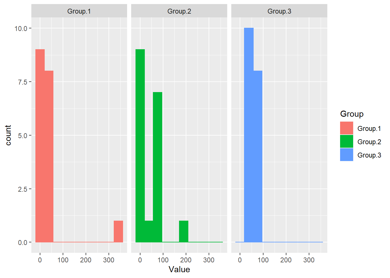
# ## first install required packages if needed
#
# if(!require(dplyr)){install.packages("dplyr")}
# if(!require(FSA)){install.packages("FSA")}
# if(!require(DescTools)){install.packages("DescTools")}
# if(!require(multcompView)){install.packages("multcompView")}
Note that the equal variance assumption seems to be violated here as well as the normality assumption.
Let’s first try a one-way ANOVA and verify these assumption violations.
model <- lm(Value~Group,data=Data)

summary(model)   # no treatment effects
##
## Call:
## lm(formula = Value ~ Group, data = Data)
##
## Residuals:
## Min 1Q Median 3Q Max
## -42.50 -29.25 -16.00 17.25 298.50
##
## Coefficients:
## Estimate Std. Error t value Pr(>|t|)
## (Intercept) 4.350e+01 1.254e+01 3.468 0.00107 **
## GroupGroup.2 3.553e-15 1.774e+01 0.000 1.00000
## GroupGroup.3 7.105e-15 1.774e+01 0.000 1.00000
## ---
## Signif. codes: 0 '***' 0.001 '**' 0.01 '*' 0.05 '.' 0.1 ' ' 1
##
## Residual standard error: 53.21 on 51 degrees of freedom
## Multiple R-squared: 1.017e-31, Adjusted R-squared: -0.03922
## F-statistic: 2.594e-30 on 2 and 51 DF, p-value: 1anova(model) # looks a little weird## Analysis of Variance Table
##
## Response: Value
## Df Sum Sq Mean Sq F value Pr(>F)
## Group 2 0 0.0 0 1
## Residuals 51 144413 2831.6layout(matrix(1:4,nrow=2,byrow=T))
plot(model) # notice the outliers! And violation of normality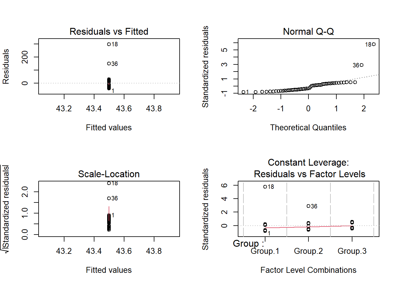
shapiro.test(residuals(model))##
## Shapiro-Wilk normality test
##
## data: residuals(model)
## W = 0.59012, p-value = 4.93e-11Okay let’s run a K-W test then!
# K-W test

kruskal.test(Value ~ Group, data = Data)   # now there is a significant group effect!
##
## Kruskal-Wallis rank sum test
##
## data: Value by Group
## Kruskal-Wallis chi-squared = 7.3553, df = 2, p-value = 0.02528Of course, now you’d want to know which groups differ from which other groups. For this we need pairwise comparisons. The most common pairwise comparison test to accompany the K-W test is the Dunn test.
library(FSA) # make sure you have this package installed!## ## FSA v0.9.3. See citation('FSA') if used in publication.
## ## Run fishR() for related website and fishR('IFAR') for related book.dt = dunnTest(Value ~ Group,data=Data,method="bh")
dt## Dunn (1964) Kruskal-Wallis multiple comparison## p-values adjusted with the Benjamini-Hochberg method.## Comparison Z P.unadj P.adj
## 1 Group.1 - Group.2 -1.356036 0.17508782 0.17508782
## 2 Group.1 - Group.3 -2.712071 0.00668642 0.02005926
## 3 Group.2 - Group.3 -1.356036 0.17508782 0.26263172Now we could add our compact letter display- in which case we would want to indicate that group 3 differs from group 1. So group 1 could get an “a”, group 2 could get an “ab”, and group 3 could get a “b”.
An alternative to the Dunn test is to use pairwise Mann-Whitney U (MWU) tests and then to use a Bonferroni correction (or another similar correction) to control the experiment-wise error rate.
In the above example, we would run three MWU tests- one for each pairwise comparison- and would reject the null if any of the p-values was less than \(\frac{\alpha}{3}\) (applying the Bonferroni correction).
Power analysis?
Perhaps we can run a power analysis example in a future iteration of this class. In the meantime let’s move on to generalized linear models and mixed-effects models.
FINAL NOTE: design-based vs model-based inference
In this class I have emphasized the equivalence between ANOVA and regression. This is because I lean on the side of ‘model-based inference’ vs ‘design-based inference’.
ANOVA is closely linked with experimental design. If you control for all confounding variables so that your categorical “treatment” is the only factor that could influence your response process, you can run an ANOVA and you are home free- there is nothing left to do- you have your answer in hand. This is called design-based inference because you designed your experiment to control for nuisance variables that could limit your inference. This makes the statistical analyses easy! Design based inference uses careful experimental design to control for nuisance factors.
However, in observational studies we often can’t control for nuisance factors using experimental design. Instead we often need to control for nuisance factors within our model. This process is called model-based inference. Model based inference is often not as satisfying, more difficult, and often much less powerful, and prone to subtle and pernicious errors, and requiring more complex statistics, etc., BUT it is often the best we can do!! Because this class is for ecologists and environmental scientists, I tend to emphasize model-based inference over design-based inference. And this is why I de-emphasize ANOVA and instead emphasize linear regression, glm, and mixed models (lmer, glmm).
This is the subject of the next lecture.