Data Generating Models
NRES 746
Fall 2025
NOTE: click here for the companion R-script for this lecture.
Why simulate ‘fake data’?
- Formalize your understanding of the data generating process (make
your assumptions explicit)
- if you can tell a computer how to do it, you REALLY understand it!
- it forces you to confront any underlying assumptions head-on
- it allows you to better understand the implications of your hypotheses (every model you build is essentially a hypothesis)
- Assess how sampling methods potentially affect information recovery
- Power Analysis! (how likely am I to pick up important signals from
this sampling design?)
- Sampling design! (what sampling design(s) will most effectively
allow me to address my research question?)
- Generate sampling distributions (e.g., bootstrap confidence intervals, CLT exercise, brute force z-test)
- Power Analysis! (how likely am I to pick up important signals from
this sampling design?)
- Assess goodness-of-fit (could your data have been produced by this
model?)
- Prior predictive check (in Bayesian stats, make sure your priors are reasonable)
- Posterior predictive check (in Bayesian stats, make sure your posterior “looks like” your actual data)
- Test whether model-fitting algorithms and statistical tests do what you think they should (e.g., estimate parameters correctly)! (test for bias, precision, etc.)
- Build intuition and proficiency for developing likelihood functions!
We have simulated data already (e.g., CLT, brute-force z-test)! Even bootstrapping is a type of data simulation…
Random number generators (sample “data” from known distributions)
Any probability distribution can be thought of as a number generator.
A discrete distribution produces whole numbers in proportion to the probability mass associated with each number in its support.
A continuous distribution produces numbers with a fractional component in proportion to the infinitessimal probability mass associated with tiny disjoint intervals within the support of the distribution.
In R, random number generator functions start with the letter ‘r’. The first argument: n, is the number of random draws you want. This argument is followed by the parameters of the distribution:
# Random number generators  -------------------------------

runif(1,0,25)   # draw random numbers from various probability distributions
rpois(1,3.4)
rnorm(1,22,5.4)
Short exercise #1:
- Generate 50 samples from \(X \sim
N(10,4.1)\)
- Generate 1000 numbers from \(X \sim
Poisson(5.4)\)
- Generate 10 numbers from \(X \sim Beta(0.1,0.1)\)
# Short exercise:

# Generate 50 samples from Normal(mean=10,sd=4.1)


# Generate 1000 samples from Poisson(mean=5.4)


# Generate 10 samples from Beta(shape1=0.1,shape2=0.1)


# Try some other distributions and parameters.  NOTE: you can visualize probability densities easily using the "curve" function. or in ggplot:

library(ggplot2)
ggplot() +
  stat_function(fun = dnorm,
                args = list(mean = 10, sd = 2.5),
                color = "red",
                linewidth = 2) +
  xlim(c(0,20)) +
  labs(x="X",y="Prob. Density") +
  theme_classic()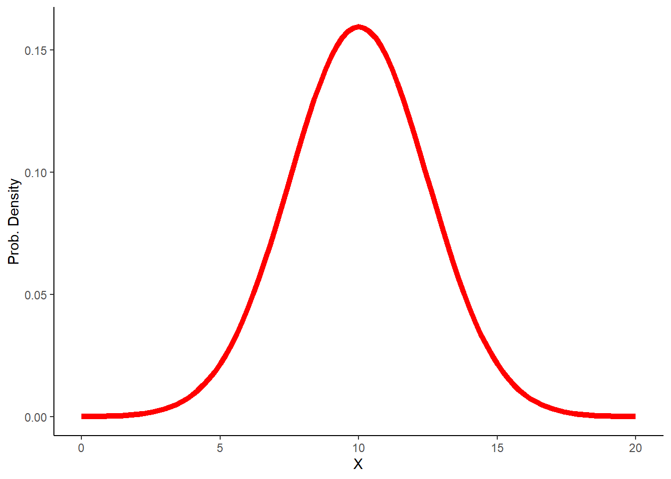
# curve(dnorm(x,0,2),-10,10)   # base R version is simpler in this case...

# What happens when you try to use a discrete distribution?
Building a data generating model
For our purposes, a data generating model is any fully specified, stochastic, computer program/script for data generation.
Your data simulation model could be as simple as the random numbers you were just generating. For example, we could make an assumption that our sample data were independently generated from a random Poisson process with constant mean (\(\lambda\)):
\[X \sim Pois(\lambda)\]
In general, our simulation models will comprise both deterministic and stochastic components.
For example, the data generating model underlying linear regression consists of a deterministic component (\(y = ax + b\)) and a stochastic component (the residual error is independently drawn from a normal distribution):
\[\mathbf{\hat{\mu}} = \mathbf{X} \mathbf{\beta}\]
\[Y_i \sim Normal(\hat{\mu_i},\sigma_{\epsilon})\] Because the variance of a normal distribution is independent from the mean, these two components can be thought of as two separate components of our data generating model.
decomposing ordinary linear regression:
First, let’s look at the deterministic component. The deterministic component maps covariate (predictor variable, or independent variable) values to an expected response \(\mu\). It is deterministic because the answer will be the same every time, given any specific input (covariate) value(s):
\[\hat{\mu}_i = \alpha +\mathbf{x}_i \cdot \mathbf{\vec\beta}\]
OR, for the univariate case:
\[\hat{\mu}_i = \alpha + \beta x_i\]
# SIMULATE DATA: ------------------
#  decompose into deterministic and stochastic components (linear regression example)

## Deterministic component  -----------------------------------------

#   define function for transforming a predictor variable into an expected response (linear regression)

    # Arguments:
      # x: vector of covariate values (predictor variable)
      # a: the intercept of a linear relationship mapping the covariate to an expected response
      # b: the slope of a linear relationship mapping the covariate to an expected response

deterministic_component <- function(x,a,b) {a + b*x}   # specify a deterministic, linear functional form

xvals = seq(0,100,5)  # define the values of a hypothetical predictor variable (e.g., tree girth)

expected_vals <- deterministic_component(xvals,175,-1.5)   # use the deterministic component to determine the expected response (e.g., tree volume)
expected_vals
## [1] 175.0 167.5 160.0 152.5 145.0 137.5 130.0 122.5 115.0 107.5 100.0 92.5
## [13] 85.0 77.5 70.0 62.5 55.0 47.5 40.0 32.5 25.0plot(xvals,expected_vals,ylab="response mean", xlab="predictor", type="l") # plot out the relationship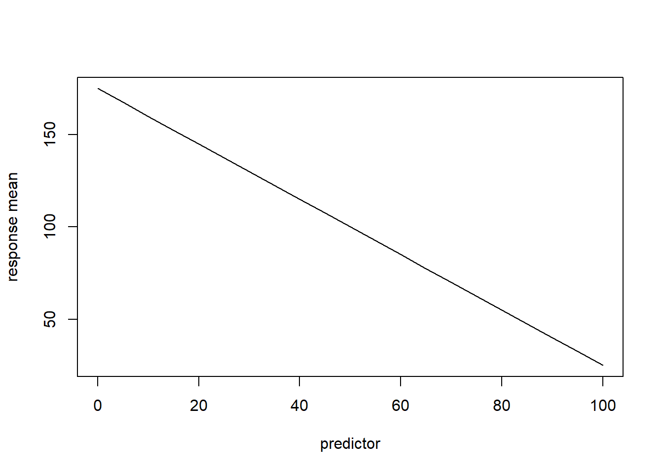
# plot(xvals,expected_vals,type="l") # alternatively, plot as a lineNow, let’s look at the stochastic component (also known as the “noise”) as a Normal distribution with standard deviation \(\sigma\):
\[Y_i \sim Normal(\hat{\mu_i},\sigma_{\epsilon})\]
You will also see this set of equations for representing a linear regression:
\[\hat{\mu}_i = \alpha + \beta x_i + \epsilon_i\] \[\epsilon_i \sim Normal(0,\sigma_{\epsilon})\]
We can consider the deterministic component as representing the expected (mean) response value given the covariate vector for unit i.
Since a normal distribution is fully defined by its mean and variance, this is is now a fully specified model.
## Stochastic component --------------------------------------------
##    define a function for transforming an expected (deterministic) response and adding a layer of "noise" on top!

    # Arguments:
      # x: vector of expected responses
      # sd: standard deviation of the "noise" component epsilon
stochastic_component <- function(x,sd){ rnorm(length(x),x,sd)}       # add a layer of "noise" on top of the expected response values

    ### Simulate stochastic data!!
sim_vals <- stochastic_component(expected_vals,sd=10)   # try it- run the function to add noise to your expected values.

plot(xvals,sim_vals)     # plot it- it should look much more "noisy" now!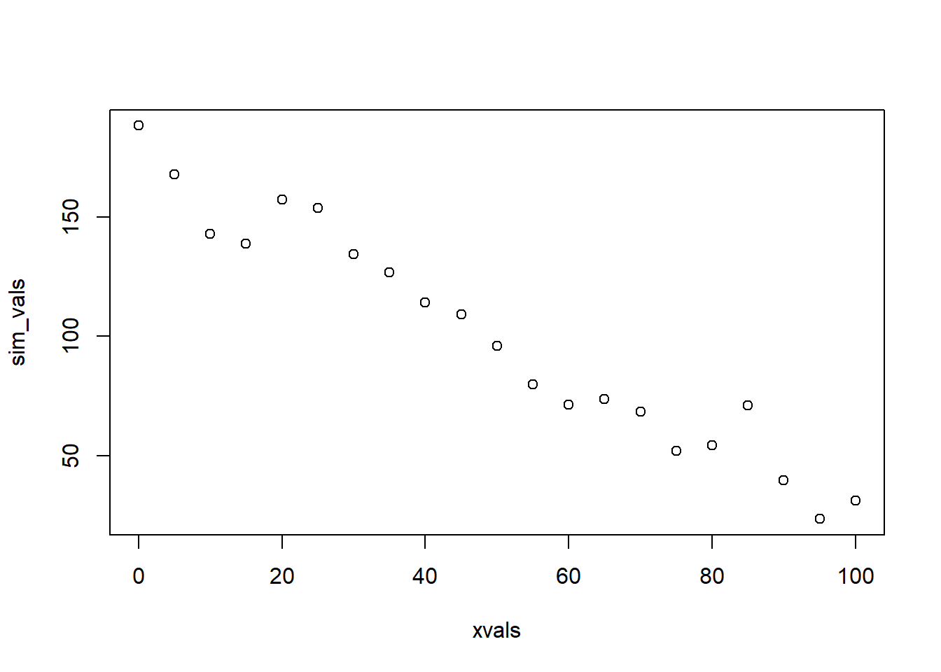
# ALTERNATIVELY:

sim_vals <- stochastic_component(deterministic_component(xvals,175,-1.5),10)    # stochastic "shell" surrounds a deterministic "core"
You can think of the deterministic component as the “signal” and the stochastic component as the “noise”.
Much of statistics and machine learning involves trying to tease apart these components– i.e., to detect signals from ‘noisy’ data.
Replication!
Okay, we’ve now generated a random data set…
But wherever there is randomness (stochasticity), we can get different results every time (that’s what it means to be random!). However, if we run lots of replicates we can gain a pretty good handle on the implications of our data generating process.
The distribution of simulated data across many replicates becomes the real result!
Goodness-of-fit
A goodness-of-fit test asks the question: can this model plausibly generate the observed data? If a data-generating model can generate data that ‘looks like’ our observations, the data-generating model passes the ‘plausibility test’.
For example, consider a set of “real” data:
# Goodness-of-fit test! -------------------------------------

    # Do the data fall into the range of plausible values produced by this model?

# Imagine you have the following "real" data (e.g., tree volumes).

realdata <- data.frame(Volume=c(0.4, 2.7, 5.3, 13.3, 42.4, 63.5, 45.8, 233.4, 213.7, 383.1),Girth=seq(1,10,length=10))
plot(realdata$Girth,realdata$Volume)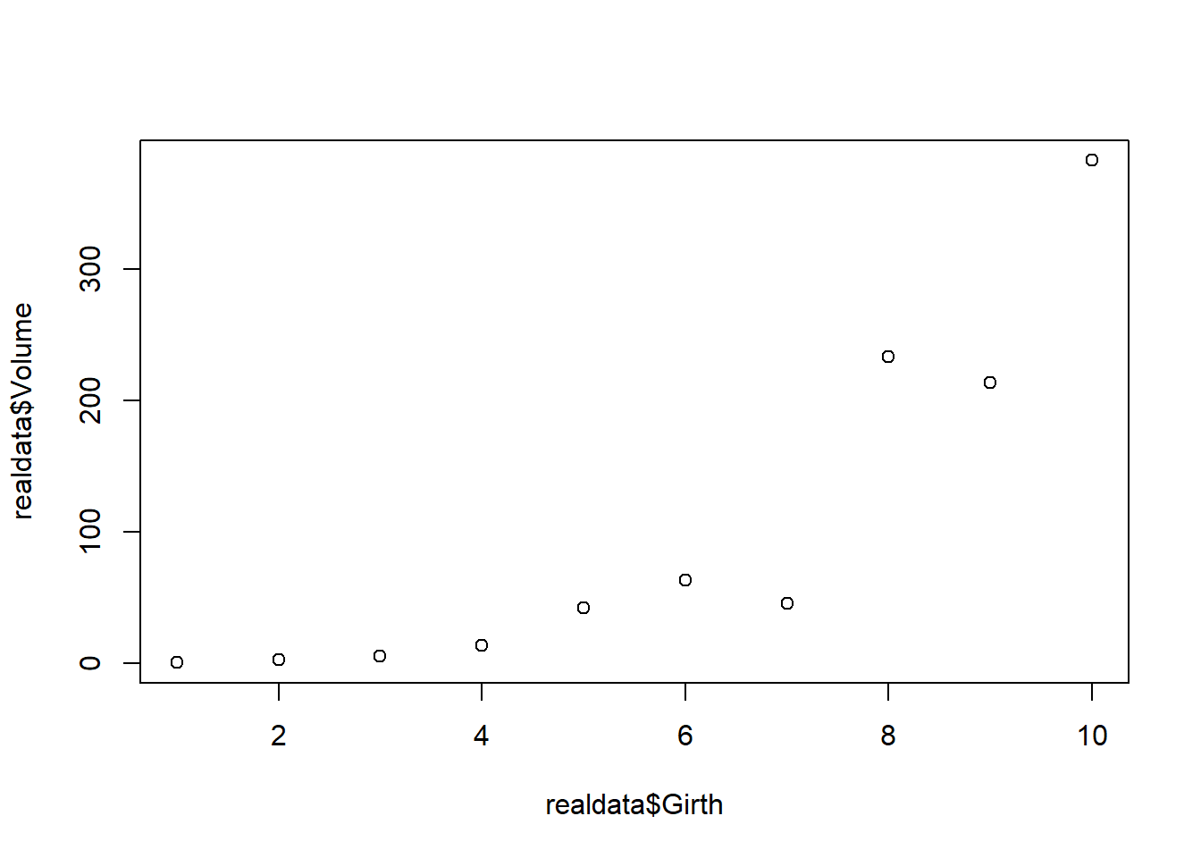
The following parameters together fully specify a data-generating model that we hypothesize is the true model that generated our data. Is this fully specified linear regression model a good fit to our data?
intercept (a) = 10         # these parameters together specify a model that hypothetically could have generated our data
slope (b) = 45
sd(sd) = 31
We can evaluate this question by generating data.
First we specify the data generating model. Then we simulate multiple datasets under this model that are comparable to our observed dataset (same sample size). Then we visually evaluate whether our data generating model is plausible.
\[Volume_i \sim Normal(\alpha + \beta x_i, \sigma_{\epsilon})\]
# Simulate many datasets from our hypothesized data generating model (intercept=10,slope=4,variance=1000):

lots <- 1000    # specify number to approximate infinity
N <- nrow(realdata)    # define the number of data points we should generate for each simulation "experiment"

simresults = replicate(lots, rnorm(N,10+realdata$Girth*40,31))

    # now make a boxplot of the results
boxplot(t(simresults),xaxt="n",ylab="Volume",xlab="Girth")    # (repeat) make a boxplot of the simulation results
axis(1,at=c(1:N),labels=realdata$Girth) # add x axis labels 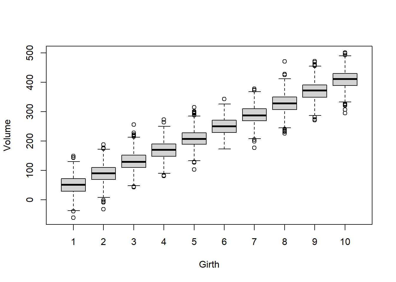
Now let’s overlay the “real” data. This gives us a visual goodness-of-fit test!
# Now overlay the "real" data
    # how well does the model fit the data?

boxplot(t(simresults),xaxt="n",ylab="Volume",xlab="Girth")    # (repeat) make a boxplot of the simulation results
axis(1,at=c(1:N),labels=realdata$Girth)                          # add x axis labels
points(c(1:N),realdata$Volume,pch=20,cex=3,col="red",xaxt="n") # this time, overlay the "real" data 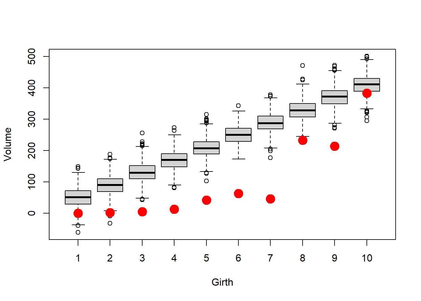
How well does this model fit the data?
Is this model likely to produce these data? (we will revisit this concept more quantitatively when we get to likelihood-based model fitting!)
What about if we try an intercept-only null model with expected Volume of 200 and sd of 400 ? What happens now?
# Let's simulate many datasets from a 'null' model (intercept=100,slope=0,sd=400):

simresults = replicate(lots, rnorm(N,100,400))
boxplot(t(simresults),xaxt="n",ylab="Volume",xlab="Girth")    # (repeat) make a boxplot of the simulation results
axis(1,at=c(1:N),labels=realdata$Girth)                          # add x axis labels
points(c(1:N),realdata$Volume,pch=20,cex=3,col="red",xaxt="n") # this time, overlay the "real" data 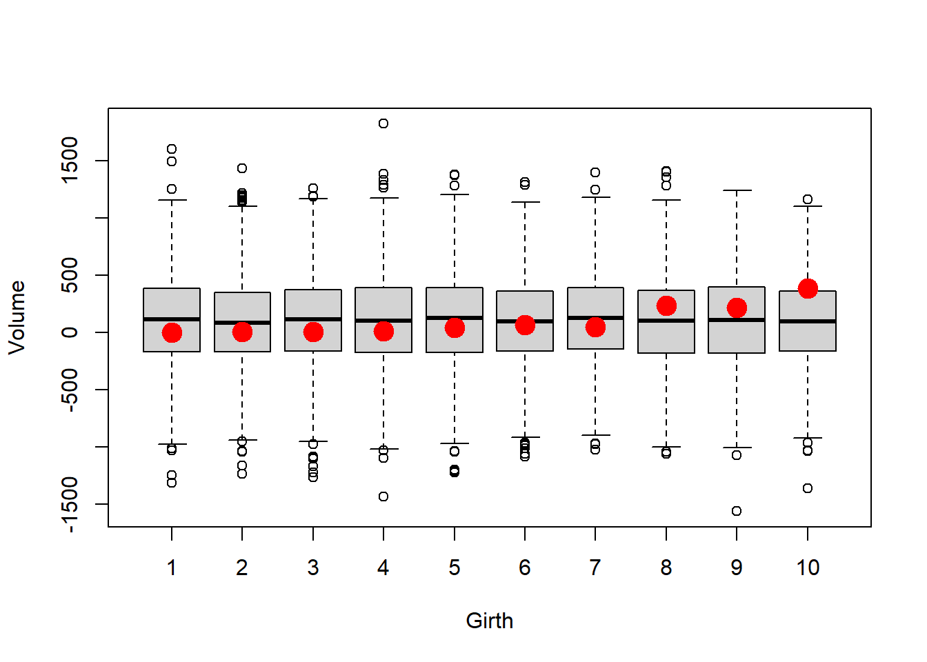
Could this model have generated the data?
What is the probability that this is the model that generated the data? What’s your intuition?
All models are wrong. Some are useful. Is this model useful?
Revisiting the tree example
Okay, let’s get real. Tree volume should not be a linear function of its girth. You learned the formula for the volume of a cylinder - how can you apply this formula here?
Linear regression and statistics in general should not be a substitute for thinking about your problem. Try to avoid thinking about statistics until you have thoroughly thought through your data and your system. Draw a DAG, think about mechanistic relationships. Statistics only comes at the end.
Generating sampling distributions (i.e., simulate the distribution of summary statistics under a null hypothesis)
A null hypothesis can nearly always be expressed as a data-generating model.
If so, you should be able to generate sampling distributions of any test statistic under your assumed null distribution.
For example, the ‘brute force’ z-test from the first lecture!
NOTE: Frequentist statistical tests are based on a random sample from a large population of possible data observations.
The interpretation of the results is based on the idea of sampling variability. You need to imagine hypothetical sample replication.
E.g., “if the null hypothesis were true, and the experiment were replicated lots and lots of times, results as or more extreme than the observed results could be expected from less than 1% of replicates”
Power analysis!!
As we prepare to run an experiment, we might ask: “is my sampling design ‘powerful’ enough detect the signal?”
We often want answers to questions like:
- What sample size do I need to be able to effectively test my hypothesis?
- What is the smallest effect size I can reliably detect with my sampling design?
- What sources of sampling or measurement error should I make the greatest effort to minimize?
In such cases, probably the most straightforward (yet not always the most efficient) way to address these questions is to generate simulated data under various sampling strategies and signal/noise ratios, and see how often you can recover the true signal through the noise!
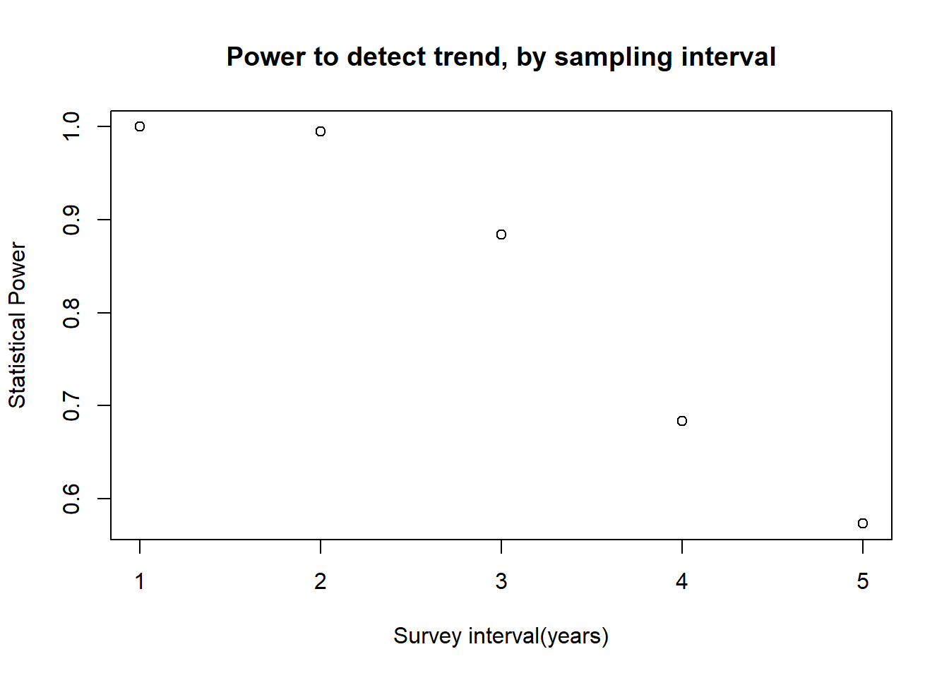
Power analysis example
Imagine we are designing a monitoring program for a population of an at-risk species, and we want to have at least a 75% chance of detecting a decline in abundance of 15% or more over a 25 year period. Let’s assume that we are using visual counts, and that the probability of encountering each member of the population is 2% per person-day. The most recent population estimate was 1000: here we assume that is known with certainty.
What we know:
- A single surveyor has a 2% chance of detecting each animal in the
population per day
- The initial abundance is 1000
- We need to detect a decline as small as 15% over 25 years with at least 75% probability
First, let’s set the groundwork by making some helper functions (break the problem into smaller chunks).
This function takes the true number in the population and returns the observed number:
# Power analysis example ---------------------------------
#    designing a monitoring program for a rare species


   ### first, let's develop some helper functions:

## helper function 1 ---------------------------
# function for computing the probability of observing each animal in a single multi-day, multi-observer survey

    # Arguments:
      # N: population abundance
      # people: number of survey participants each day
      # days: survey duration, in days
      # pObs: prob of detection per person per day

SurvProb <- function(N=1000,people=1,days=3,pObs=0.02){
  probPerDay <- 1-(1-pObs)^people      # define the probability of detection per animal per day
  1-(1-probPerDay)^days       # define the probability of detection per animal for the entire survey
}
SurvProb(500,people=2,days=7,pObs=0.02)   # test the new function
## [1] 0.2463581This function will simulate a single dataset (time series of observations over a given number of years)!
## function: simulate monitoring data ----------------------------

# develop a function for simulating monitoring data from a declining population

    # Arguments:
      # N0: true initial population abundance
      # trend: proportional change in population size from last year
      # nyears: duration of simulation
      # people: number of survey participants each day
      # days: survey duration, in days
      # survint: survey interval, in years (e.g., 2 means surveys are conducted every other year)

SimulateMonitoringData <- function(N0=1000,trend=-0.03,nyears=25,people=1,days=3,survint=2){
  realAbund <- floor(N0 * (1+trend)^(0:(nyears-1)))   # no fractional individuals
  detected <- sapply(realAbund, function(t)  rbinom(1,t, SurvProb(t,people=people,days=days,pObs=0.02)   ) )
  detected[!c(0:(nyears-1))%%survint==0] <- NA            # if the survey is not performed that year, return a missing value
  detected       # return the number of individuals detected
}

SimulateMonitoringData(N0=1000,trend=-0.03,nyears=25,people=1,days=3,survint=4)    # test the new function
## [1] 58 NA NA NA 51 NA NA NA 39 NA NA NA 39 NA NA NA 35 NA NA NA 31 NA NA NA 27Note that we are using NA to indicate years where no survey was conducted. A zero value would mean something very different than an NA.
Now we can develop a function for determining if a decline was in fact detected by the method:
## function: assessing whether or not a decline was detected ------------------------

    # Arguments:
      # monitoringData: simulated results from a long-term monitoring study
      # alpha: define acceptable type-I error rate (acceptable false positive rate)

IsDecline <- function(monitoringData,alpha=0.05){
  time <- 1:length(monitoringData)      # vector of survey years
  model <- lm(monitoringData~time)    # for now, let's use ordinary linear regression (perform linear regression on simulated monitoring data)
  p_value <- summary(model)$coefficients["time","Pr(>|t|)"]      # extract the p-value
  isdecline <- ifelse(summary(model)$coefficients["time","Estimate"]<0,TRUE,FALSE)     # determine if the simulated monitoring data determined a "significant" decline
  sig_decline <- ifelse((p_value<=alpha)&(isdecline),TRUE,FALSE)    # if declining and significant trend, then the monitoring protocol successfully diagnosed a decline
  return(sig_decline)
}

IsDecline(monitoringData=c(10,20,NA,15,1),alpha=0.05)    # test the function
## [1] FALSENow we can develop a “power” function that gives us the statistical power for given monitoring scenarios…
This is part of this week’s lab assignment!
## Review lab exercise (lab 2) ----------------------------
##     develop a "power" function to return the statistical power to detect a decline under alternative monitoring schemes...

GetPower <- function(N0,trend,nyears,people,days,survint,alpha){
     # fill this in!
  return(Power)
}
And we can evaluate what types of monitoring programs might be acceptable: