Model Performance Evaluation

Click here for the companion R script for this lecture.

In this course so far, we have constructed data-generating models and fitted these models to observed data using likelihood-based methods (ML and Bayesian inference). We also have explored a range of methods to account for structural uncertainty (which of a set of candidate models could plausibly have generated our observed data).

But even after we have fitted a model to data, even after we have compared a suite of plausible models and selected the best one, are we really sure that the model is good?

What does it even mean to say that the model is good?

Usually, we mean one or more of the following:

1. Goodness-of-fit: The data could easily/reasonably have been generated under the fitted model (the model is adequate)
2. Predictive performance: The fitted model performs well at predicting responses for out-of-sample data (the model is useful)
3. Generality: The model performs well at extrapolating responses for out-of-sample data that are outside the range of those in the training set (the model is really useful!)

Goodness-of-fit

We have already looked at a variety of methods for evaluating goodness-of-fit. In general, you can use data simulation to evaluate whether your fitted model is capable of generating the observed data. In a frequentist/ML context this is often called a parametric bootstrap.

Q: What is the difference between a non-parametric bootstrap (usually just called a ‘bootstrap’) and a parametric bootstrap?

For example, we can overlay the observed data (or a model performance statistic like R-squared) on a cloud of points representing the range of data sets (or performance statistics) possibly produced under the fitted model.

Or, we can use a “plug-in” prediction bounds as a substitute for the cloud of data sets possibly produced under the model.

Often, we compare a target summary statistic (e.g., Deviance, RMSE, R-squared) for the observed data with the range of that target summary statistic produced under the inferred, stochastic data generating model.
Let’s return to the Myxomatosis dataset!

library(emdbook)

MyxDat <- MyxoTiter_sum
Myx <- subset(MyxDat,grade==1)  #Data set from grade 1 of myxo data
head(Myx)

##   grade day titer
## 1     1   2 5.207
## 2     1   2 5.734
## 3     1   2 6.613
## 4     1   3 5.997
## 5     1   3 6.612
## 6     1   3 6.810

Now let’s use ML to fit the Ricker model with a gamma error distribution.

# Fit the model with ML -----------------------------

Ricker <- function(a,b,predvar) a*predvar*exp(-b*predvar)
  
NLL_myx <- function(params){
  expected <- Ricker(params[1],params[2],Myx$day)
  -sum(dgamma(Myx$titer,shape=expected*params[3],rate=params[3],log = T))
}

params <- c(a=1,b=0.2,rate=1)
NLL_myx(params)

## [1] 148.653

opt <- optim(params, NLL_myx)

MLE = opt$par
maxlik = opt$value

MLE

##          a          b       rate 
##  3.4735099  0.1674244 14.4243053

How might we evaluate goodness-of-fit in this case??

‘Plug-in’ prediction bounds

The simplest way is just to plot the expected value along with “plug-in” bounds around that prediction, to represent the range of data likely to be produced under the model. We have done this before!

# Plug-in prediction interval -------------------------

plot(Myx$titer~Myx$day,xlim=c(0,10),ylim=c(0,15))
expected <- Ricker(MLE['a'],MLE['b'],1:10)
points(1:10,expected,type="l",col="green")

upper <- qgamma(0.975,shape=expected*MLE['rate'],rate=MLE['rate'])
lower <- qgamma(0.025,shape=expected*MLE['rate'],rate=MLE['rate'])

points(1:10,upper,type="l",col="red",lty=2)
points(1:10,lower,type="l",col="red",lty=2)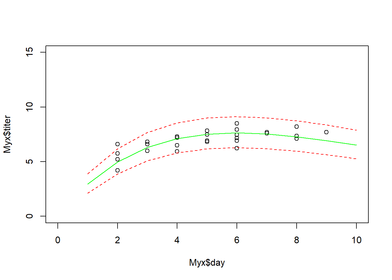

This gives us a simple and useful way to visualize goodness-of-fit.

Simulated datasets!

Alternatively, we could generate simulated data sets under the best-fit model (parametric bootstrap- essentially the same thing as the plug-in prediction interval above):

# Parametric bootstrap!  -------------------------------------

plot(Myx$titer~Myx$day,xlim=c(0,10),ylim=c(0,15),type="n")
expected <- Ricker(MLE['a'],MLE['b'],1:10)
points(1:10,expected,type="l",col="darkgreen")

uniquedays <- sort(unique(Myx$day))
expected <- Ricker(MLE['a'],MLE['b'],uniquedays)

simdata = t(replicate(1000,rgamma(length(uniquedays),shape=expected * MLE['rate'],rate=MLE['rate'])))

upper <- apply(simdata,2,function(t) quantile(t,0.975))
lower <- apply(simdata,2,function(t) quantile(t,0.025))

points(uniquedays,upper,type="l",col="red",lty=2)
points(uniquedays,lower,type="l",col="red",lty=2)

boxplot(x=as.list(as.data.frame(simdata)),at=uniquedays,add=T,boxwex=0.25,xaxt="n",range=0,col="red")
points(Myx$day,Myx$titer,cex=1.5,pch=20)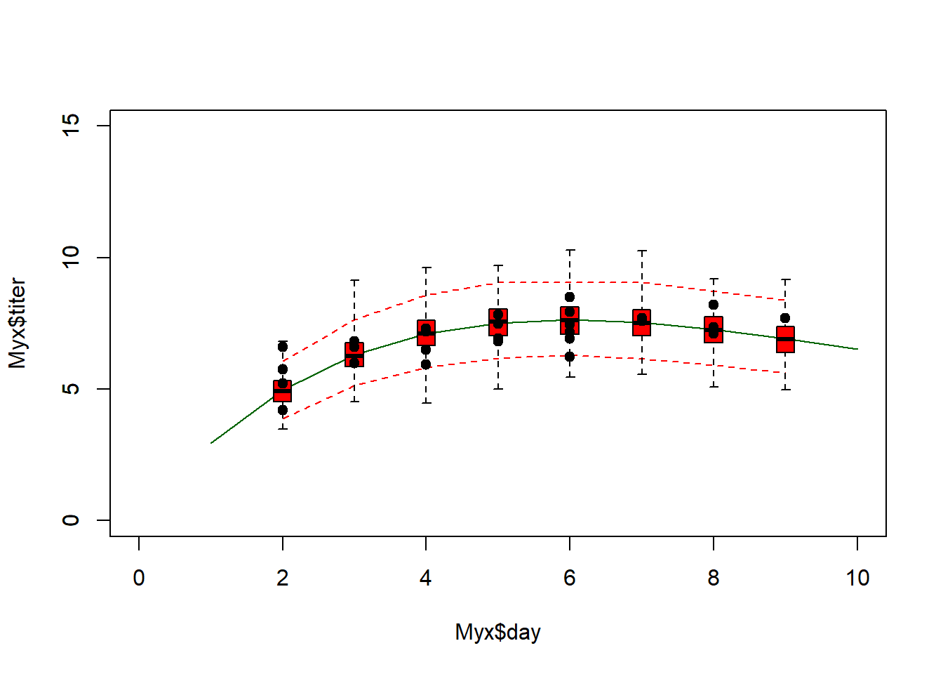

Using simulated data, we can go further- we can compare the simulated data vs the observed data more quantitatively. For example, we can compute the root mean squared error (RMSE) for the simulated datasets and compare that with the root mean squared error for the observed data. Alternatively, we could use the deviance statistic instead of RMSE.

# Compare observed error statistic with expected range of error statistic as part of parametric bootstrap analysis

expected <- Ricker(MLE['a'],MLE['b'],Myx$day)
simdata = t(replicate(1000,rgamma(length(Myx$day),shape=expected * MLE['rate'],rate=MLE['rate'])))
 
rmse_observed <- sqrt(mean((Myx$titer-expected)^2))
rmse_simulated <- apply(simdata,1,function(t) mean((t-expected)^2))

hist(rmse_simulated,freq=F)
abline(v=rmse_observed,col="darkgreen",lwd=3)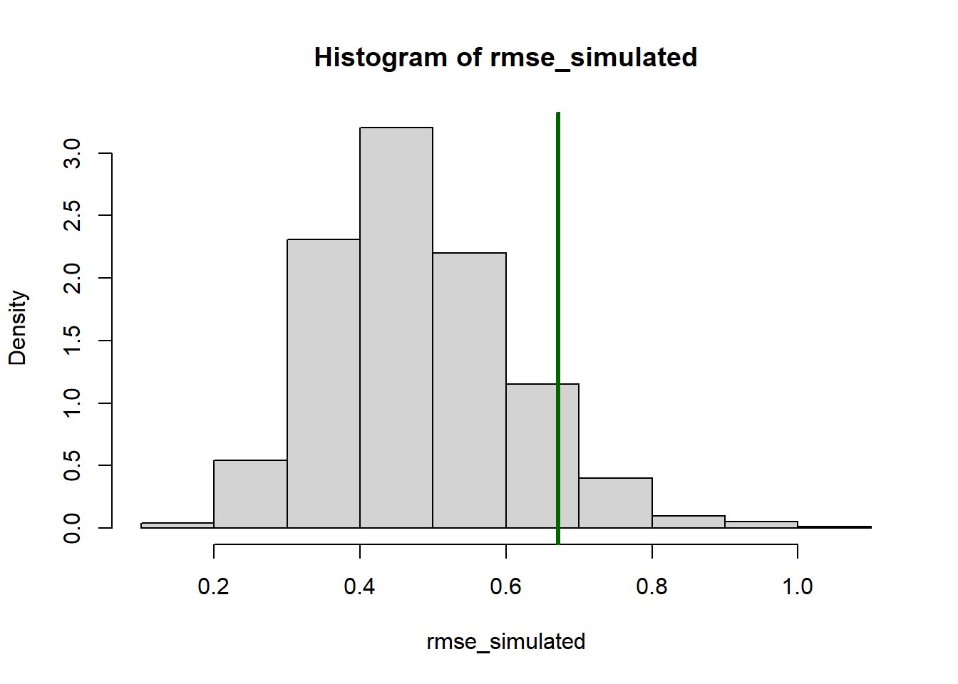

So, is this a good model?

Of course, the goodness-of-fit tests you can run with simulated data are limited only by your imagination!

NOTE: the above methods do not account for parameter uncertainty. This model is the maximum likelihood model- that is, the point estimates are assumed to represent the true model!

If we wanted to account for parameter uncertainty in the ML framework, we could (for example) use profile-likelihood CIs to estimate parameter bounds and we could plug-in bounds that incorporate parameter uncertainty. Or we could treat the CIs for the parameter estimates as a probability distribution (e.g., uniform) and simulate datasets across this range of parameter uncertainty (but what would a frequentist statistician say about this?).

Bayesian!

Accounting for prediction uncertainty is simple in a Bayesian framework… (this is part of lab 4!)

In general, a posterior predictive check involves generating new data sets under the fitted model that are equivalent to the observed data set (i.e., same sample size and covariate values) and comparing with the observed data.

First we need to fit the model in stan.

Let’s first load up the packages and set global options.

# Bayesian goodness-of-fit  -------------------------

library(cmdstanr)

## This is cmdstanr version 0.9.0

## - CmdStanR documentation and vignettes: mc-stan.org/cmdstanr

## - CmdStan path: C:/Users/kshoemaker/.cmdstan/cmdstan-2.37.0

## - CmdStan version: 2.37.0

library(posterior)

## This is posterior version 1.6.1

## 
## Attaching package: 'posterior'

## The following objects are masked from 'package:stats':
## 
##     mad, sd, var

## The following objects are masked from 'package:base':
## 
##     %in%, match

library(bayesplot)

## This is bayesplot version 1.14.0

## - Online documentation and vignettes at mc-stan.org/bayesplot

## - bayesplot theme set to bayesplot::theme_default()

##    * Does _not_ affect other ggplot2 plots

##    * See ?bayesplot_theme_set for details on theme setting

## 
## Attaching package: 'bayesplot'

## The following object is masked from 'package:posterior':
## 
##     rhat

options(mc.cores=4)

Here’s the stan code for the basic myxomatosis/gamma case:

data {
  int<lower=0> N;
  vector[N] titer;
}

parameters {
  real<lower=0> shape;
  real<lower=0> rate;
}

model {
  shape ~ gamma(0.001,0.001);   // prior on shape
  rate ~ gamma(0.001,0.001);   // prior on rate
  titer ~ gamma(shape, rate);   // likelihood
}

Let’s run the model with a ricker function for allowing titer to change as a function of time since infection.

# test your stan code:

mod1 <- cmdstan_model("myx2.stan") # Compile stan model

stan_data <- list(   # bundle data for stan
    N = nrow(Myx),
    titer = Myx$titer,
    day=Myx$day
)

fit <- mod1$sample(
  data = stan_data,
  chains = 4,
  iter_warmup = 500,
  iter_sampling = 500,
  refresh = 0   # don't provide progress updates
)

## Running MCMC with 4 parallel chains...

## Chain 1 Informational Message: The current Metropolis proposal is about to be rejected because of the following issue:

## Chain 1 Exception: gamma_lpdf: Shape parameter[1] is inf, but must be positive finite! (in 'C:/Users/KSHOEM~1/AppData/Local/Temp/RtmpUDoLxR/model-4d54444a17e8.stan', line 19, column 2 to column 29)

## Chain 1 If this warning occurs sporadically, such as for highly constrained variable types like covariance matrices, then the sampler is fine,

## Chain 1 but if this warning occurs often then your model may be either severely ill-conditioned or misspecified.

## Chain 1

## Chain 2 Informational Message: The current Metropolis proposal is about to be rejected because of the following issue:

## Chain 2 Exception: gamma_lpdf: Shape parameter[1] is inf, but must be positive finite! (in 'C:/Users/KSHOEM~1/AppData/Local/Temp/RtmpUDoLxR/model-4d54444a17e8.stan', line 19, column 2 to column 29)

## Chain 2 If this warning occurs sporadically, such as for highly constrained variable types like covariance matrices, then the sampler is fine,

## Chain 2 but if this warning occurs often then your model may be either severely ill-conditioned or misspecified.

## Chain 2

## Chain 1 finished in 0.2 seconds.
## Chain 2 finished in 0.2 seconds.
## Chain 3 finished in 0.2 seconds.
## Chain 4 finished in 0.2 seconds.
## 
## All 4 chains finished successfully.
## Mean chain execution time: 0.2 seconds.
## Total execution time: 0.5 seconds.

fit$summary()

## # A tibble: 85 × 10
##    variable    mean  median     sd    mad      q5     q95  rhat ess_bulk
##    <chr>      <dbl>   <dbl>  <dbl>  <dbl>   <dbl>   <dbl> <dbl>    <dbl>
##  1 lp__     -29.6   -29.2   1.41   1.10   -32.3   -28.2    1.00     658.
##  2 a          3.48    3.48  0.222  0.213    3.11    3.84   1.00     703.
##  3 b          0.168   0.168 0.0115 0.0112   0.149   0.186  1.00     716.
##  4 rate      12.9    12.6   3.55   3.45     7.64   19.5    1.00     903.
##  5 m[1]       4.98    4.98  0.214  0.204    4.62    5.33   1.00     750.
##  6 m[2]       4.98    4.98  0.214  0.204    4.62    5.33   1.00     750.
##  7 m[3]       4.98    4.98  0.214  0.204    4.62    5.33   1.00     750.
##  8 m[4]       6.31    6.31  0.212  0.204    5.96    6.66   1.00     832.
##  9 m[5]       6.31    6.31  0.212  0.204    5.96    6.66   1.00     832.
## 10 m[6]       6.31    6.31  0.212  0.204    5.96    6.66   1.00     832.
## # ℹ 75 more rows
## # ℹ 1 more variable: ess_tail <dbl>

samples <- fit$draws(format="draws_df")
bayesplot::mcmc_trace(samples,"a"); bayesplot::mcmc_trace(samples,"b")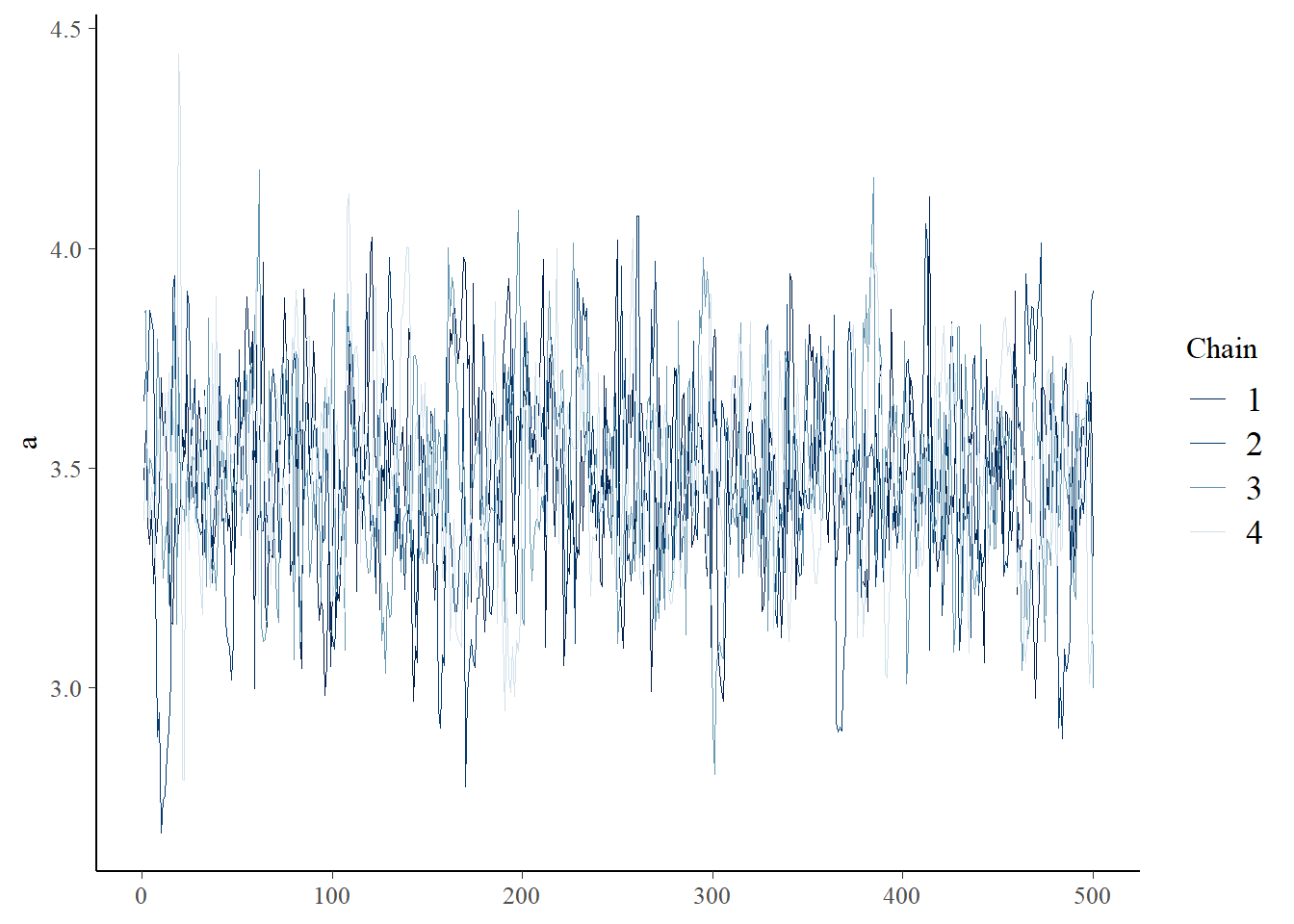

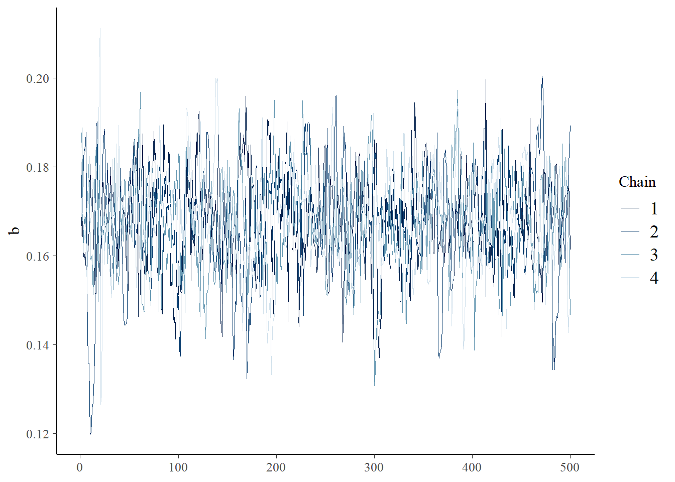
bayesplot::mcmc_trace(samples,"rate")

Assuming convergence, let’s move on to the goodness-of-fit part! First, let’s visualize the observed data against the cloud of data that could be produced under this model!

# set range of days
days=1:10

nMCMC = length(samples$a)

# make predictions from posterior
n_samp = 500
do_pred = function(){
  grab = samples[sample(1:nMCMC,1),]
  with(grab,rgamma(length(days), shape=Ricker(a,b,days)*rate,rate=rate) )
}
post_pred = as.data.frame(t(replicate(n_samp,do_pred())))

plot(Myx$titer~Myx$day,xlim=c(0,10),ylim=c(0,15),type="n")
expected <- Ricker(mean(samples$a),mean(samples$b),1:10)
points(1:10,expected,type="l",col="darkred",lwd=2)

boxplot(x=as.list(post_pred),at=1:10,add=T,boxwex=0.25,xaxt="n",range=0,border="darkred")
points(Myx$day,Myx$titer,cex=1.5,pch=20)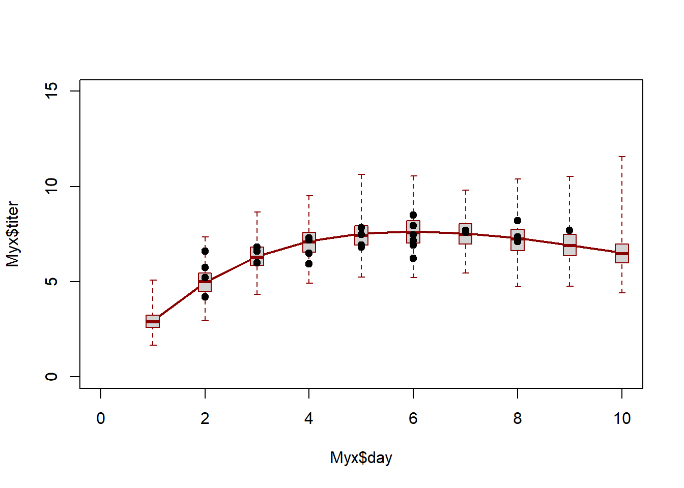

Looks pretty good so far! Let’s look at another posterior predictive check…

n_samp = 500
do_pred2 = function(){
  grab = samples[sample(1:nMCMC,1),]
  thismean = with(grab, Ricker(a,b,Myx$day))
  thissim = with(grab, rgamma(nrow(Myx),thismean*rate,rate=rate ))
  RMSE_obs = sqrt(mean((Myx$titer-thismean)^2))
  RMSE_sim = sqrt(mean((thissim-thismean)^2))
  c(RMSE_obs = RMSE_obs,RMSE_sim = RMSE_sim)
}
post_pred2 = as.data.frame(t(replicate(n_samp,do_pred2())))

plot(post_pred2$RMSE_sim~post_pred2$RMSE_obs, main="posterior predictive check")
abline(0,1,col="red",lwd=2)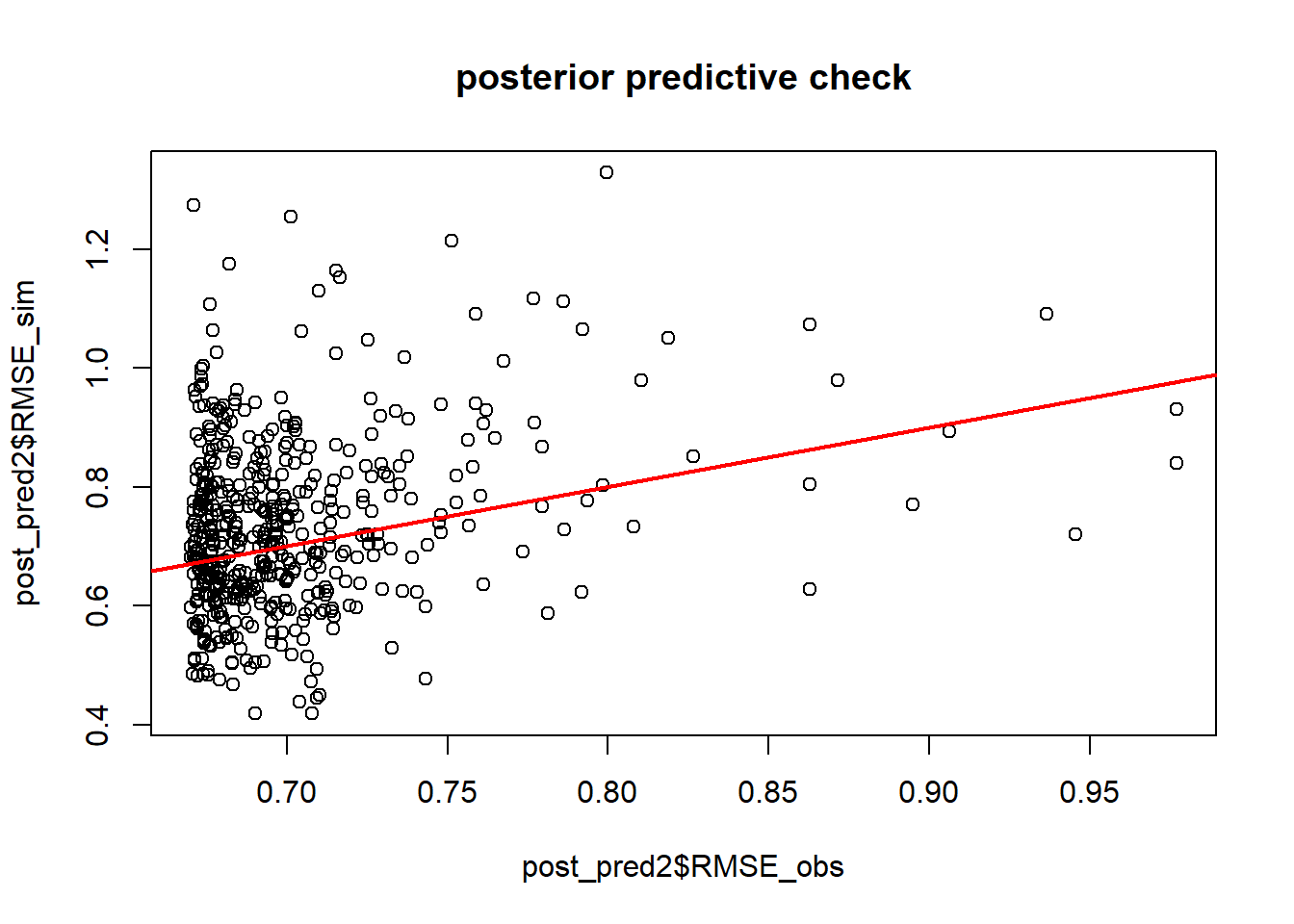

p.value=mean(post_pred2$RMSE_sim>post_pred2$RMSE_obs)
p.value

## [1] 0.546

Okay, the fit seems more or less reasonable!

Predictive ability

In many cases, goodness-of-fit is not ultimately what we are most interested in. What we really want to know is whether the model does a good job at predicting the response. Is our model useful in some way?

One way to do this would be for us to focus on an R-squared or pseudo-R2 statistic:

\[R^2 = 1-\frac{SS_{res}}{SS_{tot}}\]

\[PseudoR^2 = 1-(\frac{\ell_{mod}}{\ell_{null}})\]

Let’s compute these metrics for the fitted data:

# Summary statistics of a models "usefulness" (e.g., R-squared)  -------------------

SS_res <- sum((Myx$titer-Ricker(MLE["a"],MLE["b"],Myx$day))^2)
SS_tot <- sum((Myx$titer-mean(Myx$titer))^2)
Rsquared <- 1-SS_res/SS_tot

cat("R-squared = ", Rsquared, "\n")

## R-squared =  0.4744355

# Fit the null likelihood model!

NLL_null <- function(params){
  -sum(dgamma(Myx$titer,shape=params[1]*params[2],rate=params[2],log = T))
}

init.params <- c(mean=7,rate=1)

opt_null <- optim(par=init.params, fn=NLL_null)
MLE_null=opt_null$par
maxlik_null = opt_null$value

McFadden <- 1-(maxlik/maxlik_null)
cat("McFadden's R-squared = ", McFadden) 

## McFadden's R-squared =  0.2483471

Another way to evaluate model skill, or performance, is to use root mean squared error (RMSE):

\(RMSE = sqrt(mean(residuals^2))\)

RMSE gives a good indicator of the mean error rate, which is often useful and understandable. For example, “the predicted temperature is usually within 1.3 degrees C of the true temperature”…

RMSE = sqrt(mean((Myx$titer-Ricker(MLE["a"],MLE["b"],Myx$day))^2))
cat("RMSE = ", RMSE, "\n")

## RMSE =  0.6712301

So is our model good???

Does it do a good job at prediction?

Q: Does an over-fitted model have acceptable goodness-of-fit?

Q: Does an over-fitted model have acceptable performance, evaluated as R-squared or RMSE?

Q: Will an over-fitted model perform well when predicting to new samples (that were not used in model fitting)?

Validation

Let’s imagine we collect some new Myxomatosis titer data (for grade 1 virus), and it looks like this:

# Collect new data that were not used in model fitting

newdata <- data.frame(
  grade = 1,
  day = c(2,3,4,5,6,7,8),
  titer = c(4.4,7.2,6.8,5.9,9.1,8.3,8.8)
)
newdata

##   grade day titer
## 1     1   2   4.4
## 2     1   3   7.2
## 3     1   4   6.8
## 4     1   5   5.9
## 5     1   6   9.1
## 6     1   7   8.3
## 7     1   8   8.8

First we might simply visualize the new data against the cloud of data possibly produced under the fitted model…

# Validation #1  -------------------------

plot(Myx$titer~Myx$day,xlim=c(0,10),ylim=c(0,15),type="n",xlab="days",ylab="titer")
expected <- Ricker(MLE['a'],MLE['b'],1:10)
points(1:10,expected,type="l",col="green")

expected <- Ricker(MLE['a'],MLE['b'],1:10)
simdata <- array(0,dim=c(1000,10))
for(i in 1:1000){
  simdata[i,] <- rgamma(10,shape=expected*MLE['rate'],rate=MLE['rate'])
}

upper <- apply(simdata,2,function(t) quantile(t,0.975))
lower <- apply(simdata,2,function(t) quantile(t,0.025))

points(1:10,upper,type="l",col="green",lty=2)
points(1:10,lower,type="l",col="green",lty=2)

boxplot(x=as.list(as.data.frame(simdata)),at=1:10,add=T,boxwex=0.25,xaxt="n",range=0,border="green")
points(newdata$day,newdata$titer,cex=1.5,pch=20,col="red")
points(Myx$day,Myx$titer,cex=1.5,pch=20,col="black")
legend("topleft",pch=c(20,20),col=c("black","red"),legend=c("original data","validation data"))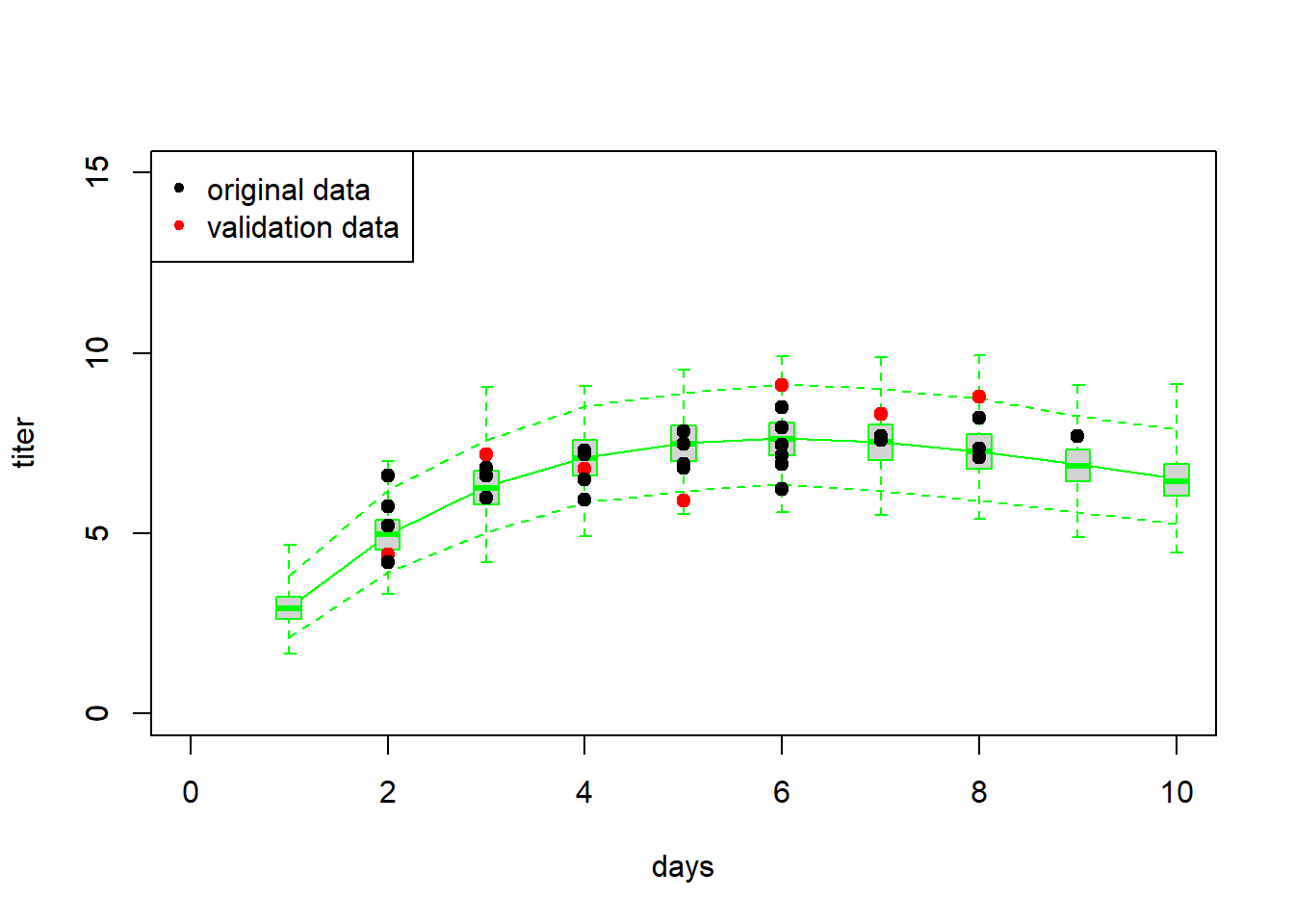

Now let’s evaluate the skill of our model at predicting the new data… using our above measures of skill, or performance.

SS_res <- sum((newdata$titer-Ricker(MLE["a"],MLE["b"],newdata$day))^2)
SS_tot <- sum((newdata$titer-mean(newdata$titer))^2)
Rsquared_validation <- 1-SS_res/SS_tot

cat("R-squared = ", Rsquared_validation, "\n")

## R-squared =  0.4787264

expected <- Ricker(MLE["a"],MLE["b"],newdata$day)
McFadden_validation <- 1-(sum(dgamma(newdata$titer,shape=expected*MLE["rate"],rate=MLE["rate"], log = T))/sum(dgamma(newdata$titer,shape=MLE_null["mean"]*MLE_null['rate'],rate=MLE_null["rate"],log=T)))
cat("pseudo R-squared = ", McFadden_validation, "\n")

## pseudo R-squared =  0.1992145

RMSE = sqrt(mean((newdata$titer-Ricker(MLE["a"],MLE["b"],newdata$day))^2))
cat("RMSE = ", RMSE, "\n")

## RMSE =  1.127411

The above analyses seem to indicate that the model fits the new data well, and that the model is successfully able to explain some of the variation in the new data.

Generality/extrapolation

Imagine we collect some more new data, this time in which titers are measured from day 10 to 16. Let’s see if the model does a good job now!

# Validation #2 ---------------------------

newdata <- data.frame(        # imagine these are new observations...
  grade = 1,
  day = c(10,11,12,13,14,15,16),
  titer = c(6.8,8.0,4.5,3.1,2.7,1.2,0.04)
)
newdata

##   grade day titer
## 1     1  10  6.80
## 2     1  11  8.00
## 3     1  12  4.50
## 4     1  13  3.10
## 5     1  14  2.70
## 6     1  15  1.20
## 7     1  16  0.04

As before, let’s first simply visualize the new data against the cloud of data possibly produced under the fitted model…

plot(Myx$titer~Myx$day,xlim=c(0,20),ylim=c(0,15),type="n",xlab="days",ylab="titer")
expected <- Ricker(MLE['a'],MLE['b'],1:20)
points(1:20,expected,type="l",col="green")

expected <- Ricker(MLE['a'],MLE['b'],1:20)
simdata <- array(0,dim=c(1000,20))
for(i in 1:1000){
  simdata[i,] <- rgamma(20,shape=expected*MLE['rate'],scale=MLE['rate'])
}

upper <- apply(simdata,2,function(t) quantile(t,0.975))
lower <- apply(simdata,2,function(t) quantile(t,0.025))

points(1:20,upper,type="l",col="green",lty=2)
points(1:20,lower,type="l",col="green",lty=2)

boxplot(x=as.list(as.data.frame(simdata)),at=1:20,add=T,boxwex=0.25,xaxt="n",range=0,border="green")
points(newdata$day,newdata$titer,cex=1.5,pch=20,col="red")
points(Myx$day,Myx$titer,cex=1.5,pch=20,col="black")
legend("topleft",pch=c(20,20),col=c("black","red"),legend=c("original data","new data"))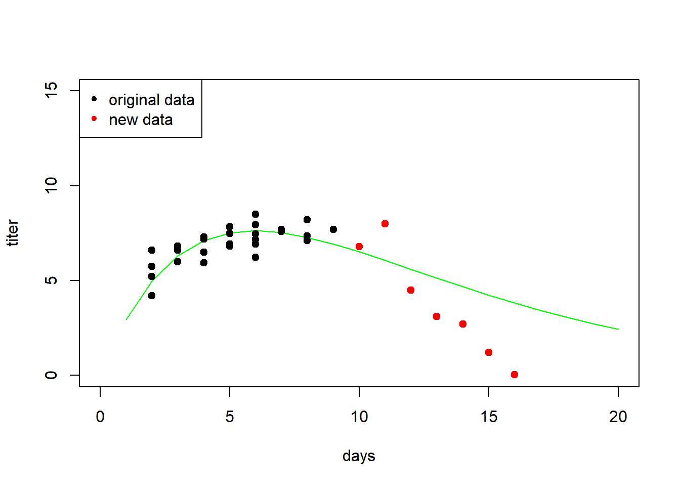

Now let’s evaluate the skill of our model at predicting the withheld data… using our favorite measures of skill, or performance.

SS_res <- sum((newdata$titer-Ricker(MLE["a"],MLE["b"],newdata$day))^2)
SS_tot <- sum((newdata$titer-mean(newdata$titer))^2)
Rsquared_validation <- 1-SS_res/SS_tot

cat("R-squared = ", Rsquared_validation, "\n")

## R-squared =  0.2674646

expected <- Ricker(MLE["a"],MLE["b"],newdata$day)
McFadden_validation <- 1-(sum(dgamma(newdata$titer,shape=expected*MLE["rate"],rate=MLE["rate"], log = T))/sum(dgamma(newdata$titer,shape=MLE_null["mean"]*MLE_null["rate"],rate=MLE_null["rate"],log=T)))
cat("pseudo R-squared = ", McFadden_validation, "\n")

## pseudo R-squared =  0.1260971

RMSE = sqrt(mean((newdata$titer-Ricker(MLE["a"],MLE["b"],newdata$day))^2))
cat("RMSE = ", RMSE, "\n")

## RMSE =  2.280982

Here are some final thoughts:

1. Models are often not very good at extrapolation.
   
2. The R-squared isn’t always the best measure of model performance.
   
3. The McFadden pseudo-Rsquared can go below 0
   
4. It’s really important to evaluate goodness-of-fit in addition to model performance!

Cross-validation

In many cases, you will not have new data against which to test the model. Cross-validation allows us to test the model anyway. Here is some pseudocode:

1. Partition the data into k partitions
2. Fit the model, leaving one data partition out at a time
   • loop through the partitions.
     
   • for each iteration of the loop, fit the model to all the data EXCEPT the observations in this partition
     
   • use this new fitted model to predict the response variable for all observations in this partition
     
3. Compute overall model performance for the cross-validation!

The most common forms of cross-validation are: (1) leave-one-out (jackknife) and (10-fold)

Let’s go through an example using the Myxomatosis data!

# CROSS-VALIDATION ------------------


# PARTITION THE DATA

n.folds <- nrow(Myx)   # jackknife

Myx$fold <- sample(c(1:n.folds),size=nrow(Myx),replace=FALSE)

init.params <- c(a=1,b=0.2,rate=1)

   # new likelihood function that takes data as an argument
NLL_myx = function(params,data){
  expected <- Ricker(params[1],params[2],data$day)
  -sum(dgamma(data$titer,shape=expected*params[3],rate=params[3],log = T))
}

Myx$pred_CV <- 0
for(i in 1:n.folds){
  Myx2 <- subset(Myx,fold!=i)   # observations to use for fitting 
  newfit <- optim(par=init.params, fn=NLL_myx, data=Myx2)   # fit the model, leaving out this partition
  ndx <- Myx$fold == i
  Myx$pred_CV[ndx] <- Ricker(newfit$par['a'],newfit$par['b'],Myx$day[ndx])
}

Myx$pred_full <- Ricker(MLE['a'],MLE['b'],Myx$day)

Myx

##    grade day titer fold  pred_CV pred_full
## 1      1   2 5.207   20 4.940054  4.970219
## 2      1   2 5.734   26 4.882567  4.970219
## 3      1   2 6.613    1 4.796755  4.970219
## 4      1   3 5.997   22 6.332117  6.306020
## 5      1   3 6.612   13 6.277516  6.306020
## 6      1   3 6.810    8 6.260143  6.306020
## 7      1   4 5.930   19 7.180973  7.111849
## 8      1   4 6.501   18 7.146799  7.111849
## 9      1   4 7.182    5 7.107221  7.111849
## 10     1   4 7.292   23 7.101235  7.111849
## 11     1   5 7.819   17 7.506576  7.519363
## 12     1   5 7.489    3 7.520617  7.519363
## 13     1   5 6.918   10 7.544845  7.519363
## 14     1   5 6.808   12 7.549647  7.519363
## 15     1   6 6.235    7 7.700272  7.632219
## 16     1   6 6.916   25 7.668105  7.632219
## 17     1   2 4.196   21 5.066275  4.970219
## 18     1   9 7.682    6 6.758880  6.927996
## 19     1   8 8.189    9 7.154969  7.280590
## 20     1   7 7.707    4 7.515624  7.531580
## 21     1   7 7.597   11 7.524418  7.531580
## 22     1   8 7.112   15 7.300420  7.280590
## 23     1   8 7.354   14 7.266284  7.280590
## 24     1   6 7.158   16 7.655622  7.632219
## 25     1   6 7.466   24 7.639953  7.632219
## 26     1   6 7.927    2 7.617211  7.632219
## 27     1   6 8.499   27 7.588721  7.632219

To assess how well the model is performing, let’s compute the root mean squared error for the full model vs the cross-validation:

RMSE_full <- sqrt(mean((Myx$titer-Myx$pred_full)^2))
RMSE_CV <- sqrt(mean((Myx$titer-Myx$pred_CV)^2))
RMSE_full

## [1] 0.6712301

RMSE_CV

## [1] 0.7294344

As expected, the RMSE is higher under cross-validation.

Is the model still okay? One way to look at this would be to assess the variance explained.

VarExplained_full = 1 - mean((Myx$titer-Myx$pred_full)^2)/mean((Myx$titer-mean(Myx$titer))^2)
VarExplained_CV = 1 - mean((Myx$titer-Myx$pred_CV)^2)/mean((Myx$titer-mean(Myx$titer))^2)
VarExplained_full

## [1] 0.4744355

VarExplained_CV

## [1] 0.3793374

Clearly the model performance is lower under cross-validation, and almost always will be! But this is also a more honest evaluation of model performance.

Example: multiple logistic regression

NOTE: example modified from here

Let’s evaluate which factors were related to surviving the titanic disaster!

You can load the titanic data example here. Alternatively you can use the ‘titanic’ package in R!

# Cross-validation: titanic disaster example!  --------------------

# titanic <- read.csv("titanic.csv",header=T)
# head(titanic)

library(titanic)  
titanic <- titanic_train

Our goal is to model the probability of surviving the titanic disaster as a function of covariates like sex, age, number of siblings or spouses on board, number of parents or children, passenger fare, etc.

Let’s first build a simple logistic regression model for this problem.

titanic2 <- na.omit(titanic)
model1 <- glm(Survived ~ Sex + scale(Age) + scale(SibSp) + scale(Parch) + scale(Fare), data=titanic2, family="binomial")    #logistic regression
summary(model1)

## 
## Call:
## glm(formula = Survived ~ Sex + scale(Age) + scale(SibSp) + scale(Parch) + 
##     scale(Fare), family = "binomial", data = titanic2)
## 
## Coefficients:
##              Estimate Std. Error z value Pr(>|z|)    
## (Intercept)    1.2071     0.1591   7.587 3.27e-14 ***
## Sexmale       -2.5334     0.2052 -12.348  < 2e-16 ***
## scale(Age)    -0.3125     0.1043  -2.996 0.002739 ** 
## scale(SibSp)  -0.3796     0.1140  -3.330 0.000868 ***
## scale(Parch)  -0.1984     0.1001  -1.982 0.047523 *  
## scale(Fare)    0.9127     0.1663   5.487 4.08e-08 ***
## ---
## Signif. codes:  0 '***' 0.001 '**' 0.01 '*' 0.05 '.' 0.1 ' ' 1
## 
## (Dispersion parameter for binomial family taken to be 1)
## 
##     Null deviance: 964.52  on 713  degrees of freedom
## Residual deviance: 695.26  on 708  degrees of freedom
## AIC: 707.26
## 
## Number of Fisher Scoring iterations: 5

Alternatively, we could write our own likelihood function!!

params <- c(
  int=1,
  male = -1,
  age = 0,
  sibsp = 0,
  parch = 0,
  fare = 0
)

LikFunc <- function(params){
  linear <- params['int'] + 
    params['male']*as.numeric(titanic2$Sex=="male") +
    params['age']*scale(titanic2$Age) +
    params['sibsp']*scale(titanic2$SibSp) +
    params['parch']*scale(titanic2$Parch) +
    params['fare']*scale(titanic2$Fare)
  logitlinear <-  1/(1+exp(-(linear)))
  -sum(dbinom(titanic2$Survived,size=1,prob = logitlinear,log=T))
}

LikFunc(params)

## [1] 459.757

MLE <- optim(fn=LikFunc,par = params)

MLE$par

##        int       male        age      sibsp      parch       fare 
##  1.1988722 -2.5318874 -0.3174421 -0.3816480 -0.2047207  0.9109768

Interesting- the results are very slightly different from the glm results…! (I’m not sure why…)

Univariate relationships

Let’s visualize the univariate relationships in this model! One way to do this is to hold all other variables at their mean value…

SibSp_range <- range(titanic$SibSp)
Parch_range <- range(titanic$Parch)
Fare_range <- range(titanic$Fare)
Age_range <- range(titanic$Age,na.rm = T)

First, let’s look at fare

### 

plot(titanic$Survived~titanic$Fare,pch=16,xlab="FARE ($)",ylab="Survived!")

predict_df <- data.frame(
  Sex = "male",
  Age = mean(titanic$Age,na.rm=T),
  SibSp = mean(titanic$SibSp),
  Parch = mean(titanic$Parch),
  Fare = seq(Fare_range[1],Fare_range[2])
)

probSurv <- predict(model1,predict_df,type="response")

lines(seq(Fare_range[1],Fare_range[2]),probSurv)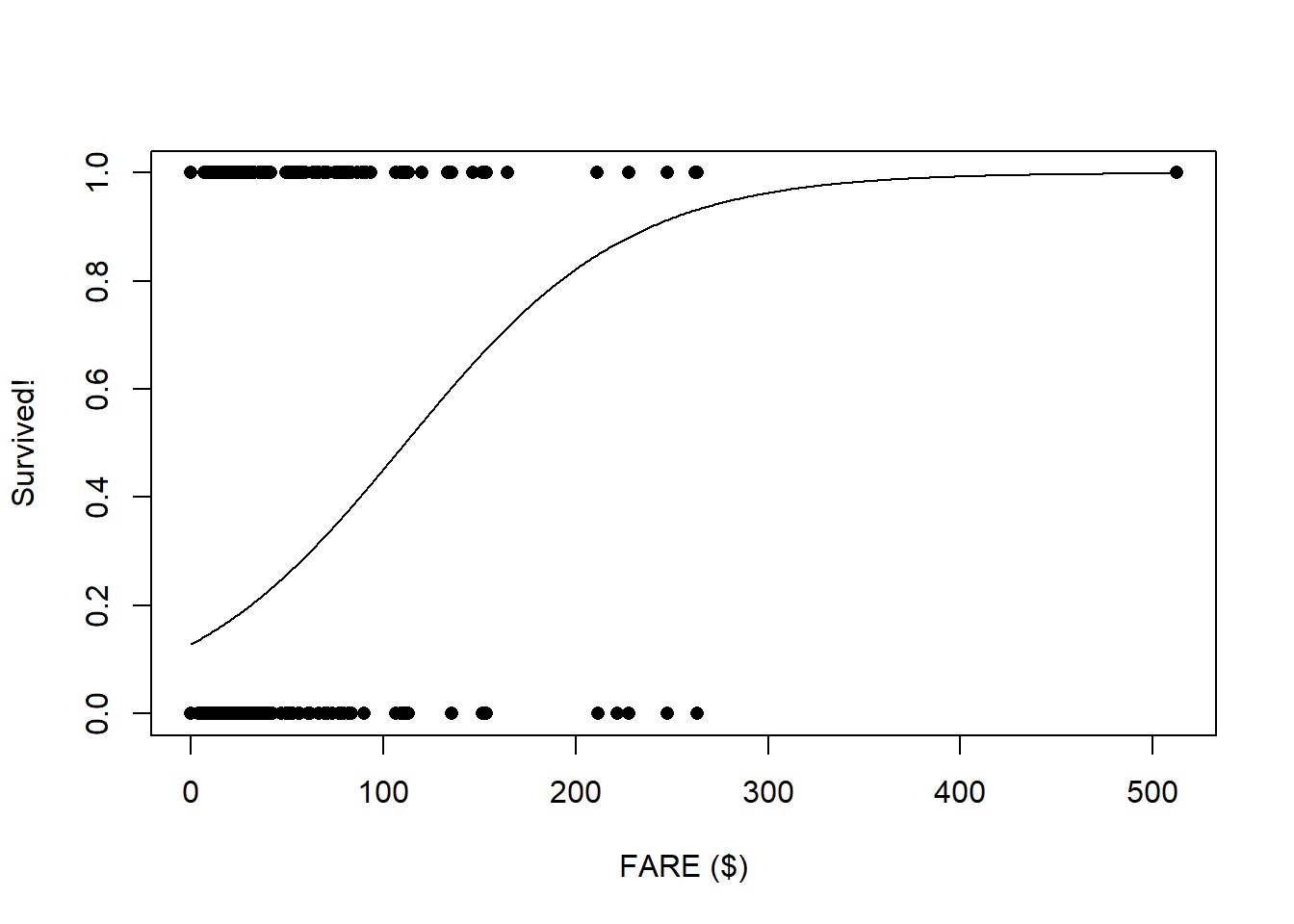

Next, let’s look at Sex:

### 

predict_df <- data.frame(
  Sex = c("male","female"),
  Age = mean(titanic$Age,na.rm=T),
  SibSp = mean(titanic$SibSp),
  Parch = mean(titanic$Parch),
  Fare = mean(titanic$Fare,na.rm=T)
)

tapply(titanic$Survived,titanic$Sex,mean)[2:1]

##      male    female 
## 0.1889081 0.7420382

probSurv <- predict(model1,predict_df,type="response")
names(probSurv) <- c("male","female")

probSurv

##      male    female 
## 0.2039291 0.7634165

Now, let’s look at age:

plot(titanic$Survived~titanic$Age,pch=16,xlab="AGE",ylab="Survived!")

predict_df <- data.frame(
  Sex = "male",
  Age = seq(Age_range[1],Age_range[2]),
  SibSp = mean(titanic$SibSp),
  Parch = mean(titanic$Parch),
  Fare = mean(titanic$Fare,na.rm=T)
)

probSurv <- predict(model1,predict_df,type="response")

lines(seq(Age_range[1],Age_range[2]),probSurv)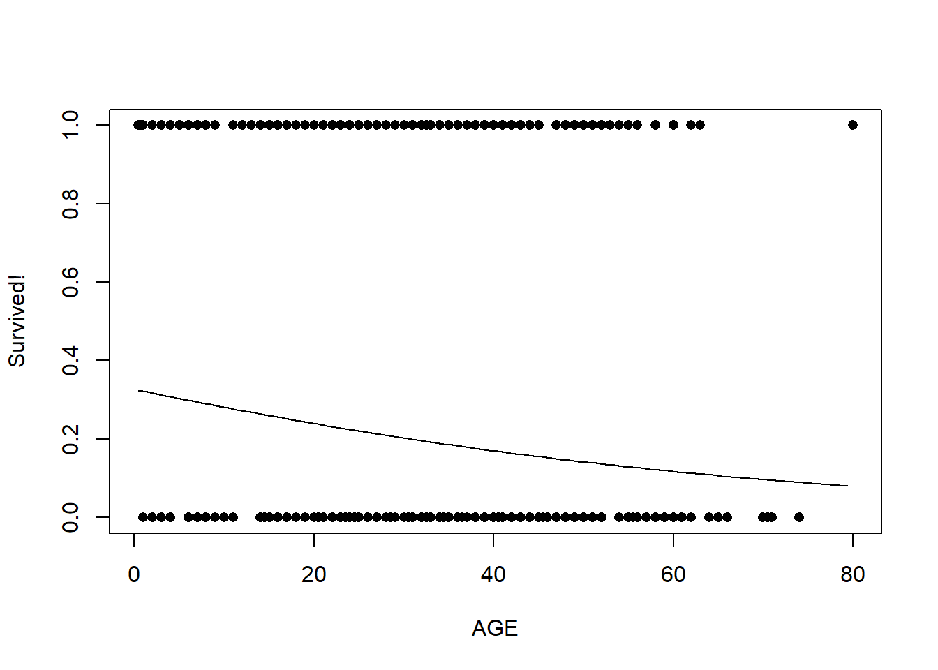

Now, let’s look at number of siblings/spouses:

### 

plot(titanic$Survived~titanic$SibSp,pch=16,xlab="# of Siblings/spouses",ylab="Survived!")

predict_df <- data.frame(
  Sex = "male",
  Age = mean(titanic$Age,na.rm=T),
  SibSp = seq(SibSp_range[1],SibSp_range[2],0.01),
  Parch = mean(titanic$Parch),
  Fare = mean(titanic$Fare,na.rm=T)
)

probSurv <- predict(model1,predict_df,type="response")

lines(seq(SibSp_range[1],SibSp_range[2],0.01),probSurv)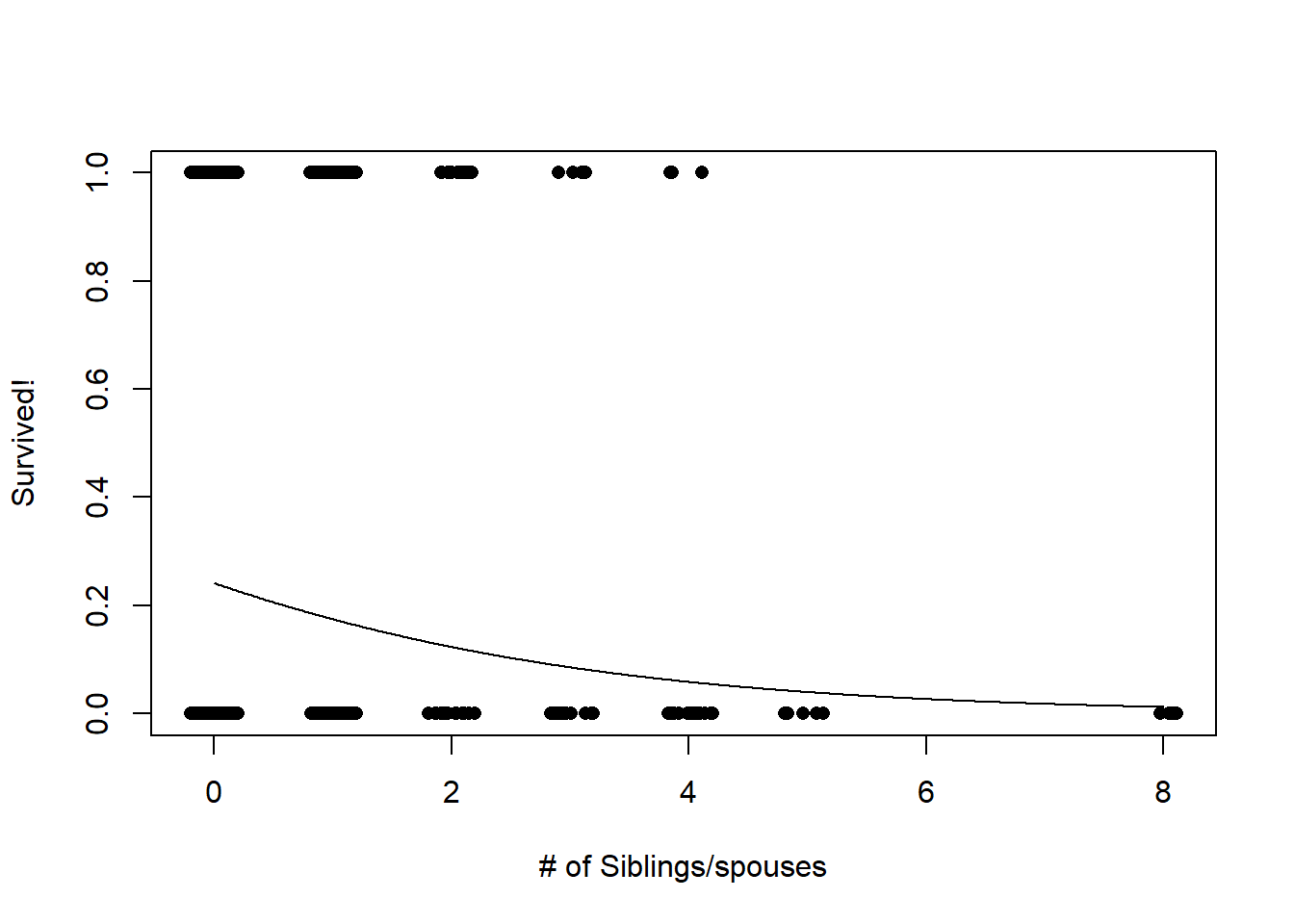

Performance evaluation / validation

Since we are interested in evaluating model performance, let’s see how well the model predicts which people survived the titanic disaster…

First of all, we will use cross-validation to evaluate model predictive performance

BUT… since the response is binary, our model skill metrics don’t really work too well!

For binary responses (0 or 1), the ROC curve (and area under the curve statistic) is a good way of evaluating model performance!

First let’s prepare the workspace- load the packages!

library(ROCR)
library(rms)

model1 <- glm(Survived ~ Sex + SibSp + Parch + Fare, data=titanic, family="binomial")

Then, we set the number of “folds” for cross-validation

# CROSS VALIDATION CODE FOR BINARY RESPONSE  ----------------------------

n.folds = 10       # set the number of "folds"
foldVector = rep(c(1:n.folds),times=floor(length(titanic$Survived)/9))[1:length(titanic$Survived)]

Then, we do the cross validation, looping through each fold of the data, leaving out each fold in turn for model training.

CV_df <- data.frame(
  CVprediction = numeric(nrow(titanic)),      # make a data frame for storage
  realprediction = 0,
  realdata = 0
)

for(i in 1:n.folds){
  fit_ndx <- which(foldVector!=i)
  validate_ndx <- which(foldVector==i)
  model <- glm(formula = Survived ~ Sex + SibSp + Parch + Fare, family = "binomial", data = titanic[fit_ndx,]) 
  CV_df$CVprediction[validate_ndx] <-  plogis(predict(model,newdata=titanic[validate_ndx,])) 
  CV_df$realprediction[validate_ndx]  <-  plogis(predict(model1,newdata=titanic[validate_ndx,]))
  CV_df$realdata[validate_ndx] <- titanic$Survived[validate_ndx]
}

CV_RMSE = sqrt(mean((CV_df$realdata - CV_df$CVprediction)^2))       # root mean squared error for holdout samples in 10-fold cross-validation
real_RMSE = sqrt(mean((CV_df$realdata - CV_df$realprediction)^2))  # root mean squared error for residuals from final model

# print RMSE statistics

cat("The RMSE for the model under cross-validation is: ", CV_RMSE, "\n")

## The RMSE for the model under cross-validation is:  0.3983029

cat("The RMSE for the model using all data for training is: ", real_RMSE, "\n")

## The RMSE for the model using all data for training is:  0.3937799

However, RMSE doesn’t have much value for binary responses like this! Here we use the ROC curve instead.

Aside: ROC curve and AUC

ROC is a useful threshold-independent metric for evaluating the performance of a binary classifier!

What does it mean to be threshold independent? It helps to look at the data we have for evaluating model performance

head(CV_df)

##   CVprediction realprediction realdata
## 1    0.1247408      0.1253180        0
## 2    0.8317980      0.8374769        1
## 3    0.7568756      0.7432668        1
## 4    0.7904207      0.7977907        1
## 5    0.1755321      0.1711690        0
## 6    0.1813810      0.1720213        0

To effectively compare our predictions with the observation we have to pick some threshold above which we call the prediction a “1” and below which it is a zero.

A threshold-independent classifier like ROC considers model performance across all possible thresholds.

Here are some example ROC curves:

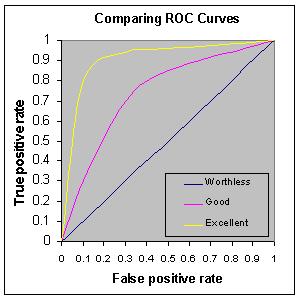
The ROC curve is generated by plotting the true positive rate against the false positive rate for all possible thresholds. For example, take the extremes:

Imagine the threshold is zero, so we predict all outcomes are a 1; that is, all people are predicted to survive the titanic disaster. In this case, the true positive rate is exactly 1 (all those that survived were predicted to survive), and the false positive rate (the rate at which mortalities were incorrectly classified as survival) is also 1!

Imagine the opposite case: we predict everyone died. In this case, the true positive rate is 0 (all those that survived were predicted to not survive), as is the false positive rate (all mortalities are correctly classified!)

Now imagine a threshold of around 0.5- we call everything above this a “1”. Now we HOPE that the observations with predictions above 0.5 are enriched in true positives relative to false positives. Maybe we get 80% correct classification of survivors and say 10 incorrect classification of mortalities (false positives).

Q What would a perfect classifier look like?

Q What would a classifier look like that performed no better than random chance?

Q What if the classifier performed worse than random chance?

Now, let’s consider the meaning of the area under the ROC curve. This is an important skill metric for a binary classifier!

Okay, back to the example! Let’s plot out the ROC curves!

par(mfrow=c(2,1))
pred <- prediction(CV_df$CVprediction,CV_df$realdata)     # for holdout samples in cross-validation
perf <- performance(pred,"tpr","fpr")
auc <- performance(pred,"auc")
plot(perf, main="Cross-validation")
text(.9,.1,paste("AUC = ",round(auc@y.values[[1]],2),sep=""))

pred <- prediction(CV_df$realprediction,CV_df$realdata)     # for final model
perf <- performance(pred,"tpr","fpr")
auc <- performance(pred,"auc")
plot(perf, main="All data")
text(.9,.1,paste("AUC = ",round(auc@y.values[[1]],2),sep=""))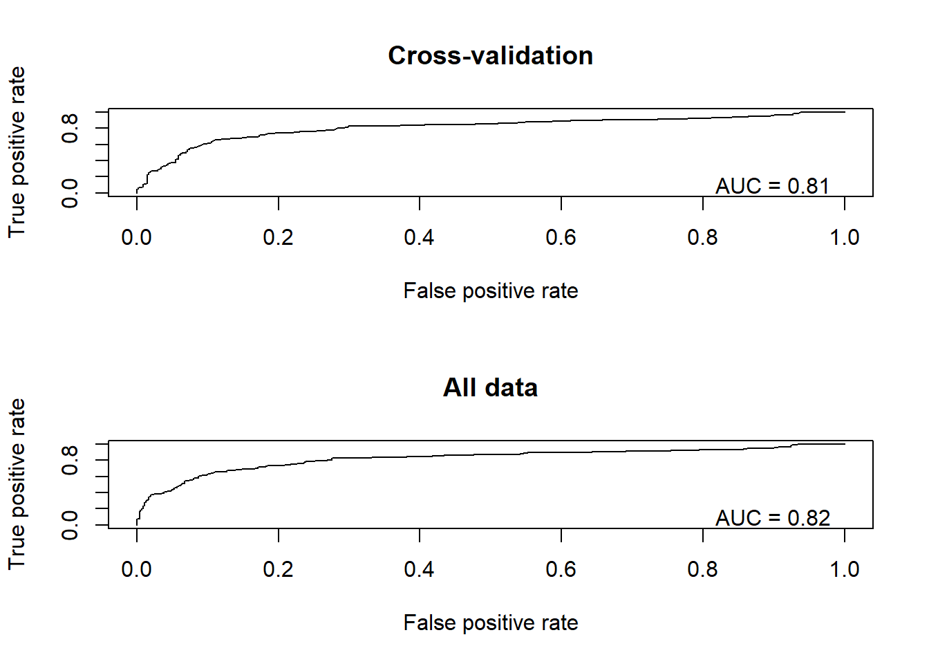

Finally, we can use the same pseudo-R-squared metric we learned above as an alternative metric of performance

CV_df$CVprediction[which(CV_df$CVprediction==1)] <- 0.9999       # ensure that all predictions are not exactly 0 or 1
CV_df$CVprediction[which(CV_df$CVprediction==0)] <- 0.0001
CV_df$realprediction[which(CV_df$realprediction==1)] <- 0.9999
CV_df$realprediction[which(CV_df$realprediction==0)] <- 0.0001

fit_deviance_CV <- mean(-2*(dbinom(CV_df$realdata,1,CV_df$CVprediction,log=T)-dbinom(CV_df$realdata,1,CV_df$realdata,log=T)))
fit_deviance_real <- mean(-2*(dbinom(CV_df$realdata,1,CV_df$realprediction,log=T)-dbinom(CV_df$realdata,1,CV_df$realdata,log=T)))
null_deviance <- mean(-2*(dbinom(CV_df$realdata,1,mean(CV_df$realdata),log=T)-dbinom(CV_df$realdata,1,CV_df$realdata,log=T)))
deviance_explained_CV <- (null_deviance-fit_deviance_CV)/null_deviance   # based on holdout samples
deviance_explained_real <- (null_deviance-fit_deviance_real)/null_deviance   # based on full model...

# print RMSE statistics

cat("The McFadden R2 for the model under cross-validation is: ", deviance_explained_CV, "\n")

## The McFadden R2 for the model under cross-validation is:  0.2564415

cat("The McFadden R2 for the model using all data for training is: ", deviance_explained_real, "\n")

## The McFadden R2 for the model using all data for training is:  0.2760832

–go to next lecture–