Module 1.1
Getting started
Spring 2026
Get materials for this module
You will be introduced to a lot of new material very quickly in this workshop, and you are not expected to remember everything! ‘Cheatsheets’ can quickly and easily refresh your memory about syntax that can be difficult to remember. So don’t worry if you don’t memorize everything we do together in this workshop- the key is that you leave this workshop with comfort working in the RStudio environment, doing some basic data operations in R, and most importantly, learning and trying new things on your own!
Here are links to good R “cheatsheets”:
Helpful packages
ggplot
cheat sheet
data
‘tidying’
data
transformation
working
with dates and times
Many additional ‘cheat sheets’ are available here
Load script for submodule #1.1
Click here to download the script for this submodule! I recommend right-clicking (or command-clicking for Macs) on the link and selecting the “Save As” option from the context menu. Save the script to a convenient folder on your laptop (e.g., a folder called “Rworkshop2023”), which will serve as your working directory for this workshop.
Start a new RStudio Project. To do this, open RStudio and from the File menu select File>>New Project. In the menu that follows, select “Existing Directory”, and then navigate to the folder in which you saved the R script for this module (your working directory). Select this folder to be your project directory. Every time you open this project (File >> Open Project), this project directory will be the first place that R looks for data files and code, and will be the default location for saving data and code.
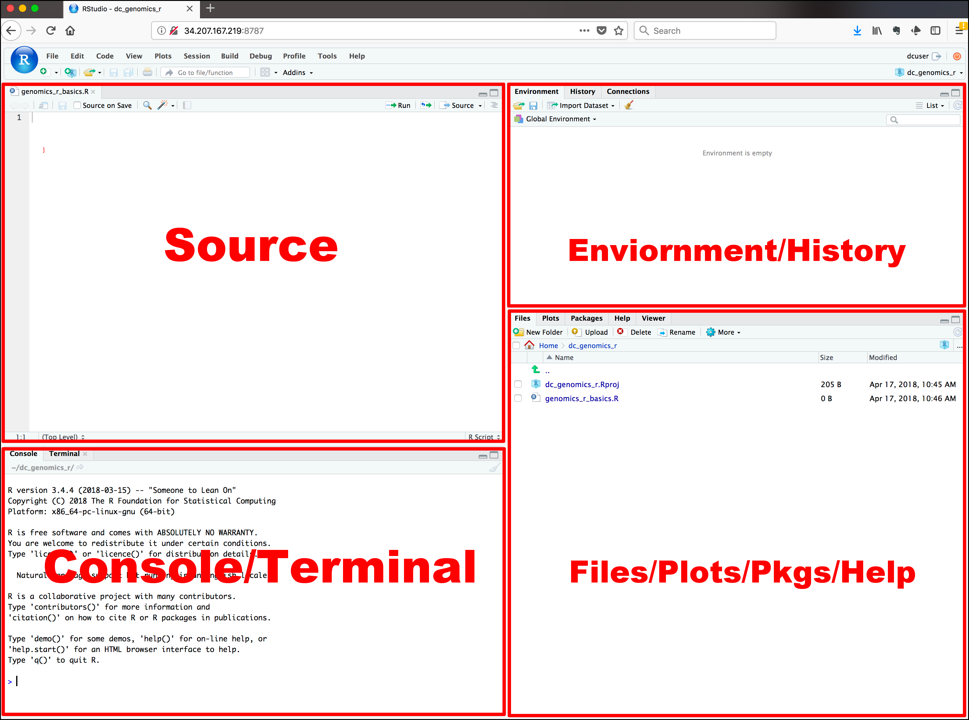
Load a blank script in RStudio. To do this, click on the “blank paper” icon at the far left of the RStudio toolbar (or File >> New File >> R script). Your RStudio interface should now be divided into four quadrants. In the RStudio default configuration, the top left panel is your script (a set of written commands that R can recognize and execute), the bottom left panel is your console (your direct connection with R), the top right panel is your environment (displays all the objects – data sets, variables, functions– that you have defined in your current R session), and the bottom right panel is a set of tabbed interfaces that let you view help files, load packages, view plots, view files in your working directory, etc.
Take a couple minutes to familiarize yourself with the RStudio environment.
Let’s get started!
Explore the R console
The R console is located in the left half or bottom left of the RStudio interface (see figure above).
The R console (what you see if you opened R directly instead of RStudio) is a command line interface, and is your direct connection with R: you give R a command at the prompt and R executes that command.
Click on the console, just to the right of one of the “>” prompts.
You can use the console like a calculator. For example, type
6+11at the prompt and hit enter.Now hit the “up” arrow. The R console remembers all previous commands that it has executed in this session, which allows you to re-run commands relatively easily.
Try typing
# 2+2and hitting “Enter”. Nothing happens, right? We will come back to the special hashtag character shortly.
Let’s create our first object
Objects are defined using R’s assignment operator
(Windows shortcut: Alt + -)(Mac: replace Alt with Option), which looks
like a left arrow (<-). Type the following statement
directly into the console:
myname <- "batman" # or use your real name. Or maybe that IS your real name...Then hit “Enter”. What does R return?
NOTHING! At least, nothing directly shows up in the console.
BUT…. check the Environment window (top right of RStudio interface- list of all the objects you’ve defined in this session). You should see that you now have a new object in your environment, called “myname”, and this object contains a single text string.
Now type myname into the R console and hit “Enter”. What
happens?
If you enter the name of an object at the command line, R automatically prints the value of the object!
NOTE: RStudio has a useful autofill feature, which can save you lots of time and headaches. After you’ve typed the first couple letters (e.g., “my”), RStudio will suggest “myname” (or use the “tab” key to trigger RStudio to give you autofill options) and you can just scroll to the right object/function and hit “Enter”! The autofill feature, unlike R, is not case sensitive!
Graduating to R Scripts
You will quickly realize that although the command-line R console is nice to use for some things (e.g., quick things that don’t need to be saved), there is a much better way to develop R code. That is by storing a sequential set of commands as a text file.
This text file (the standard is to use the “.R” extension) is called an R script.
Make a new script
If you haven’t done it already, create a new R script by clicking on the “blank paper” icon at the far left of the RStudio toolbar (or File>>New File>>R script). The top left quadrant of the RStudio interface (the “Source” window) should now contain a blank R script.
In your blank script, let’s define a new object. For example:
my_obj <- 6+11
Now place the cursor somewhere within the line of text you just wrote and hit ‘Ctrl+Enter’ (or ‘Command+Enter’) to run that line of code! You should see a new object (‘my_obj’) pop up in your environment.1.
Take a few minutes to get comfortable running commands and defining new objects using your new R script.
Of course, it’s always a good idea to save your scripts often – so feel free to save your new script before you move on.
Load an Existing script
Remember the file you downloaded at the beginning of this submodule? That file is an R script (“module1_1.R”); Let’s load it up now! You can have multiple scripts open at the same time- they appear as tabs at the top of the script/source window.
To do this, click on the “folder” icon on the Rstudio toolbar (or File >> Open File) and choose the script you downloaded earlier.
The first couple lines of the script for this module are preceded by hash marks. As you have already seen, R ignores these lines (anything preceded by a hash is ignored)- they are called comments, and they help to keep code organized and understandable.
use comments early and often- they are tremendously valuable.
Now you know the basics of how to use R scripts! Now, let’s keep working through the remainder of the script you just opened.
R Objects
Okay, let’s step back and learn a little bit about R as a data-oriented programming language.
R has many different kinds of objects that you can define and store in memory.
Objects that enable storage of information (data objects) include: vectors, matrices, lists, and data frames.
Objects that transform data and perform operations (e.g., statistics/visualizations) on data objects are called functions.
Functions
Functions are routines that take inputs (usually data objects) (also called arguments) and produce something useful in return (transformed data objects, summaries, plots, tables, statistics, files).
In R, the name of the function is followed by parentheses, and any arguments (inputs) are entered inside the parentheses. The basic syntax looks like the code snippet below.

## function syntax
functionName([argument 1, argument2, ...])
If you don’t type the parenthesis, the function is not run- instead, the function definition is shown instead.
Here are some examples of how functions are used. Note the parentheses!
# BACK TO BASICS -------------------

# functions -------------------

sum(1, 2, 3, 10)    # returns: 15

c(1, 2, 3, 10)   # combine four numbers into a single data object (construct a vector!)

floor(67.8)  # removes the decimal component of a number
round(67.8)  # rounds a number to the nearest integer
near(0.01,0,tol=0.2) # returns TRUE if argument 1 is near to argument 2 within a certain tolerance levelOops, that last one is not part of base R. It’s actually part of an R package called ‘dplyr’- one of the most commonly used packages in R ecosystem! A package is basically a set of functions that expand the capabilities of base R. Let’s load ‘dplyr’, along with a whole bunch of packages known as the ‘tidyverse’. We will also load a commonly used plotting package called ‘ggplot2’.
Using packages involved 2 steps:
1. Install the package (you only need to do this once)
2. Load the package (use the ‘library()’ function (you need to do this
every time you start a new R session).
  # load 'tidyverse'  and 'ggplot'
library(ggplot2)
library(tidyverse)
near # oops, forgot the parentheses!
near(1,1.1)
near(1,1.01)
near(1,1.000000001)
?near # get some help on this functionIt’s easy to get some help if you forget how a function works:
help(round) # a function for getting help with functions!!## starting httpd help server ... done?round # shortcut for the 'help' functionWe will revisit functions in more detail (and build our own functions) in the “Programming” submodule.
Data objects and variables
Data types
The basic data types in R are:
- “numeric” (numbers)
- “character” (text strings)
- “logical” (TRUE/FALSE)
- “factor” (categorical)
Data of each of these types can be stored in several different types of objects. We will go through them in this order:
- scalars
- vectors
- matrices
- lists
- data frames
Scalars
Scalars are the simplest data objects. A scalar is just a single value of any data type.
#  Create R Objects ------------------------


# scalars


scalar1 <- 'this is a scalar'
scalar2 <- 104
Scalars can store information of any type 2. In the example above,
scalar1 is a character, scalar2 is
numeric.
Vectors
Vectors can combine multiple scalars in a single data object.
First let’s create some vectors. In the code below we use a function
called c(). You can think of it as the ‘combine’ function-
it takes several smaller data objects and combines them together into a
single object.
# VECTORS

vector1 <- c(1.1, 2.1, 3.1, 4)   # the "c()" function combines smaller data objects into a larger object
vector2 <- c('a', 'b', 'c')
There are many different ways to create a vector. You’ll learn more about that later. Check out the vectors you just created. Each vector is composed of one or more scalar elements of the same type.
Now let’s do some stuff with vectors!
d1 <- 1:3             # make a vector: 1,2,3
d2 <- d1+3            # add 3 to all elements of the vector "myvec"
d3 <- d1+d2           # elementwise addition

length(d1)            # number of elements in a vector
sum(d3)               # sum of all elements in a vector

d2[2]                 # extract the second element in the vector

d2[2] <- 5            # change the second element in the vector
NOTE: strictly speaking, there are no true scalars in R- scalars are just vectors with 1 element!
Matrices
Matrix data objects have two dimensions: rows and columns. All of the elements in a matrix must be of the same type.
Let’s make our first matrix. One simple way to make a matrix is just
by joining two or more vectors using the function cbind()
(bind vectors or matrices together by column) or rbind()
(bind vectors or matrices together by row)
# MATRICES

mymat <- cbind(d1,d2)        # create a matrix by binding vectors, with vector d1 as column 1 and d2 as column 2
mymat
## d1 d2
## [1,] 1 4
## [2,] 2 5
## [3,] 3 6class(mymat) # confirm that the new object "mymat" is a matrix using the 'class()' function## [1] "matrix" "array"mymat <- matrix(c(1,2,3,4,5,6),nrow=3,ncol=2) # create matrix another way (matrix constructor)
mymat## [,1] [,2]
## [1,] 1 4
## [2,] 2 5
## [3,] 3 6We can do stuff with matrices:
# math with matrices
mymat + 2## [,1] [,2]
## [1,] 3 6
## [2,] 4 7
## [3,] 5 8sum(mymat)## [1] 21# extract matrix elements
mymat[3,2] # extract the element in the 3rd row, 2nd column## [1] 6mymat[,1] # extract the entire first column## [1] 1 2 3# X[a,b] access row a, column b element of matrix/data frame X
# X[,b] access all rows of column b of matrix/data frame X
# X[a,] access row a of matrix/data frame X
mymat[2,1] <- 10 # re-assign a new value to an element in a matrix
mymat[2,] <- 5 # change all elements in a row!Lists
Lists are more general than matrices. List objects are just a bunch of arbitrary R data objects (called list elements) grouped together into a single object! The elements of a list don’t need to be the same length or the same type. The elements of a list can be vectors, matrices, other lists, or even functions.
Let’s make our first list:
# LISTS
mylist <- list() # create empty list
mylist[[1]] <- c(1,2,3) # note the double brackets- this is one way to reference list elements.
mylist[[2]] <- c("foo","bar")
mylist[[3]] <- matrix(1:6,nrow=2)
mylist## [[1]]
## [1] 1 2 3
##
## [[2]]
## [1] "foo" "bar"
##
## [[3]]
## [,1] [,2] [,3]
## [1,] 1 3 5
## [2,] 2 4 6# do stuff with lists
mylist[[2]] # extract the second list element## [1] "foo" "bar"mylist[[3]][1,2] # extract the first row, second column from the matrix that is embedded as the third element in this list ! ## [1] 3mylist[[3]][1,2] <- 10 # re-assign a new value to an element of a matrix within a list!Data frames and tibbles
Data frame objects are the basic data storage object in R. Data frames are a special type of list in which each list element is a vector of equal length. Each list element in a data frame is also known as a column.
Data frames superficially resemble matrices, since both have rows and columns. However, unlike matrices, the columns of a data frame can represent different data types (i.e., character, logical, numeric, factor), and can thereby represent different types of information!
Data frames are the fundamental data storage structure in R. You can think of a data frame like a spreadsheet. Each row of the the data frame represents a different observation, and each column represents a different measurement taken on each observation unit.
Let’s make our first data frame.
# DATA FRAMES
df1 <- data.frame(col1=c(1,2,3),col2=c("A","A","B")) # create a data frame with two columns. Each column is a vector of length 3
df1## col1 col2
## 1 1 A
## 2 2 A
## 3 3 Bdf1[1,2] # extract the first element in the second column## [1] "A"df1$col2 # extract the second column by name (alternatively, df1[["col2"]])## [1] "A" "A" "B"df1$col2[2] <- 5 # reassign an element of a column of the data frame
df1$col2 <- 5 # reassign a whole column!Now we have a data frame with three observation units and two measurements (variables).
A tibble is the same thing as a data frame, just with a few tweaks to make it work better in the tidyverse. We will work with both tibbles and data frames in this workshop. For our purposes, tibbles and data frames are the same thing.
Making up data!
In this section, we will make up some fake data objects. In the next submodule we’ll practice working with real data!
Generating sequences of numbers
One task that comes up a lot is generating sequences of numbers:
# MAKING UP DATA! ----------------------------------
# Generating vector sequences
1:10 # sequential vector from 1 to 10## [1] 1 2 3 4 5 6 7 8 9 10seq(0,1,length=5) # sequence of length 5 between 0 and 1 ## [1] 0.00 0.25 0.50 0.75 1.00Another task is to group regular recurring sequences together:
# Repeating vector sequences
rep(0,times=3) # repeat 0 three times## [1] 0 0 0rep(1:3,times=2) # repeat the vector 1:3 twice## [1] 1 2 3 1 2 3rep(1:3,each=2) # repeat each element of 1:3 two times## [1] 1 1 2 2 3 3And finally, we can fill up a vector with random numbers using one of R’s built in random number generators:
# Random numbers
rnorm(10) # 10 samples from std. normal## [1] 2.62210923 0.43504596 -2.44506961 -1.06929609 -1.02425498 -0.83039892
## [7] -0.14397913 0.37943229 -0.24450319 0.09509297rnorm(10,mean=-2,sd=4) # 10 samples from Normal(-2,4^2)## [1] 0.7755803 -6.7688437 -1.9656430 0.6877746 -7.1268305 2.0898039
## [7] 0.6375658 -8.3530845 -3.7269587 -1.9444130rbinom(5,size=3,prob=.5) # 5 samples from Binom(3,0.5)## [1] 2 2 1 2 1rbinom(5,3,.1) # 5 samples from Binom(3,0.1)## [1] 0 0 1 0 0runif(10) # 10 standard uniform random numbers## [1] 0.3438716 0.7816983 0.8827020 0.4098154 0.8340670 0.5895559 0.1858751
## [8] 0.7337372 0.7468234 0.4335352runif(10,min=-1,max=1) # 10 uniform random numbers from [-1,1]## [1] 0.77267758 0.43115601 0.59635734 0.81048974 0.01898856 0.85865446
## [7] -0.85327263 -0.15918442 -0.13523707 0.09192420And finally, we can make up a fake data frame (or tibble) using some of the tricks we just learned!
# Make up an entire fake data frame!
my.data <- tibble(
Obs.Id = 1:100,
Treatment = rep(c("A","B","C","D","E"),each=20),
Block = rep(1:20,times=5),
Germination = rpois(100,lambda=rep(c(1,5,4,7,1),each=20)), # random poisson variable
AvgHeight = rnorm(100,mean=rep(c(10,30,31,25,35,7),each=20))
)
my.data## # A tibble: 100 × 5
## Obs.Id Treatment Block Germination AvgHeight
## <int> <chr> <int> <int> <dbl>
## 1 1 A 1 3 8.39
## 2 2 A 2 0 10.3
## 3 3 A 3 1 9.87
## 4 4 A 4 1 10.1
## 5 5 A 5 1 10.2
## 6 6 A 6 0 8.35
## 7 7 A 7 1 10.4
## 8 8 A 8 2 10.9
## 9 9 A 9 0 9.48
## 10 10 A 10 1 9.44
## # ℹ 90 more rowssummary(my.data) # Use the "summary()" function to summarize each column in the data frame.## Obs.Id Treatment Block Germination
## Min. : 1.00 Length:100 Min. : 1.00 Min. : 0.00
## 1st Qu.: 25.75 Class :character 1st Qu.: 5.75 1st Qu.: 1.00
## Median : 50.50 Mode :character Median :10.50 Median : 3.00
## Mean : 50.50 Mean :10.50 Mean : 3.63
## 3rd Qu.: 75.25 3rd Qu.:15.25 3rd Qu.: 5.00
## Max. :100.00 Max. :20.00 Max. :13.00
## AvgHeight
## Min. : 8.345
## 1st Qu.:24.854
## Median :29.739
## Mean :26.245
## 3rd Qu.:31.685
## Max. :36.029mydf=my.data[21:30,] # extract rows 21 to 30 and store as a new data frame
mydf## # A tibble: 10 × 5
## Obs.Id Treatment Block Germination AvgHeight
## <int> <chr> <int> <int> <dbl>
## 1 21 B 1 4 30.8
## 2 22 B 2 1 29.9
## 3 23 B 3 4 30.3
## 4 24 B 4 5 29.5
## 5 25 B 5 3 30.6
## 6 26 B 6 6 29.7
## 7 27 B 7 3 29.6
## 8 28 B 8 4 31.9
## 9 29 B 9 2 29.3
## 10 30 B 10 4 30.1mydf$Treatment # access a column of the data frame by name## [1] "B" "B" "B" "B" "B" "B" "B" "B" "B" "B"Here are some useful R functions for exploring data objects:
# Useful data exploration/checking tools in R --------------------
length(d2) # Obtain length (# elements) of vector d2
dim(mymat) # Obtain dimensions of matrix or array
summary(my.data) # summarize columns in a data frame.
names(my.data) # get names of variables in a data frame (or names of elements in a named vector)
nrow(my.data) # get number of rows/observations in a data frame
ncol(my.data) # get number of columns/variables in a data frame
str(my.data) # look at the "internals" of an object (useful for making sense of complex objects!)Challenge exercises
- Create a 3 row by 2 column matrix named ‘mymat’. Use the “rbind()” function to bind the following three rows together using these three vectors as rows:
c(1,4)
c(2,5)
c(3,6)Your final matrix should look like this:
##      [,1] [,2]
## [1,]    1    4
## [2,]    2    5
## [3,] 3 6- Create a new matrix called ‘mymat2’ that includes all the data from columns 3 to 5 of data frame mydf. HINT: use the “as.matrix()” function to coerce a data frame into a matrix.
Your result should look like this:
## Block Germination AvgHeight
## [1,] 1 4 30.76077
## [2,] 2 1 29.90424
## [3,] 3 4 30.33732
## [4,] 4 5 29.49256
## [5,] 5 3 30.62297
## [6,] 6 6 29.68407
## [7,] 7 3 29.55401
## [8,] 8 4 31.89363
## [9,] 9 2 29.26619
## [10,] 10 4 30.09393- Create a list named ‘mylist’ that is composed of a vector: 1:3, a matrix: matrix(1:6,nrow=3,ncol=2), and a data frame: data.frame(x=c(1,2,3),y=c(TRUE,FALSE,TRUE),z=c(“a”,“a”,“b”)).
Your result should look like this:
## [[1]]
## [1] 1 2 3
##
## [[2]]
## [,1] [,2]
## [1,] 1 4
## [2,] 2 5
## [3,] 3 6
##
## [[3]]
## x y z
## 1 1 TRUE a
## 2 2 FALSE a
## 3 3 TRUE bExtract the first and third observation from the 2nd column of the data frame in ‘mylist’ (the list created in challenge 6 above).
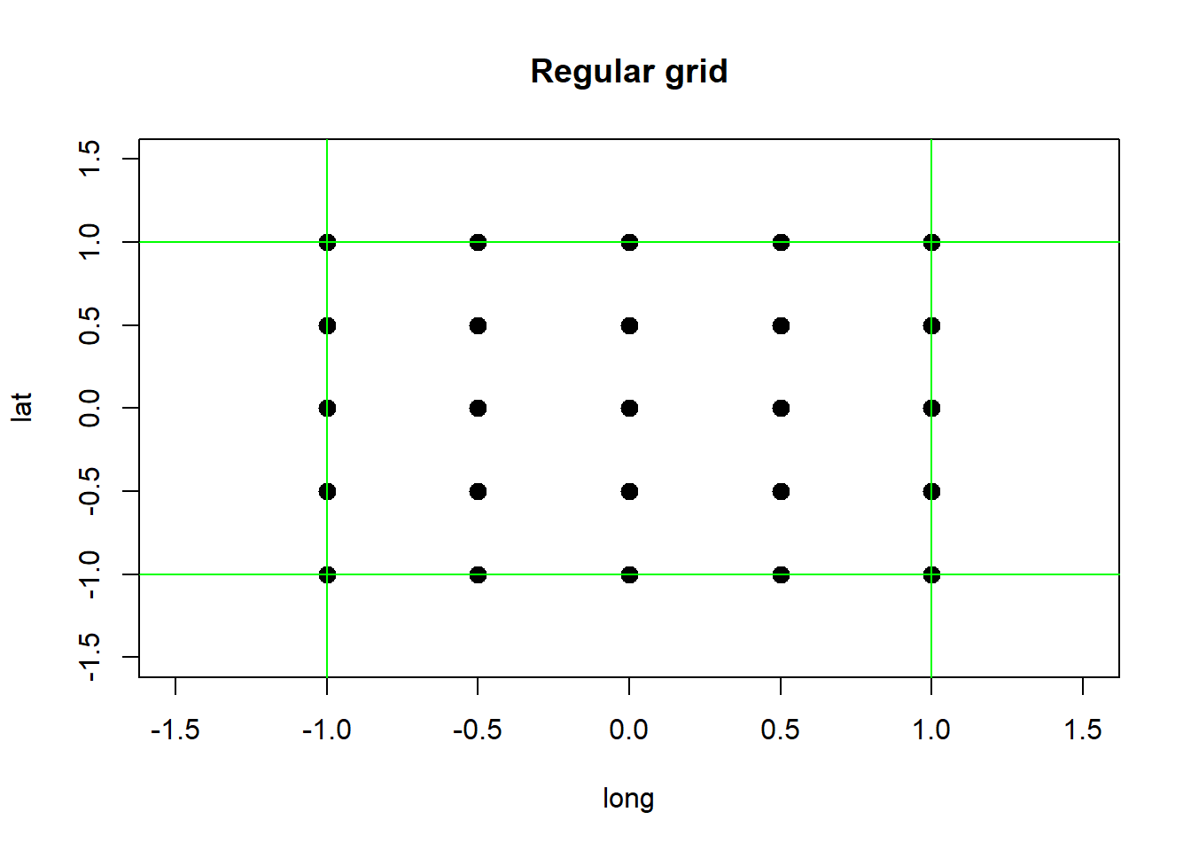
(optional- extra challenging!) Create a data frame (or tibble) named ‘df_spatial’ that contains 25 spatial locations, with ‘long’ and ‘lat’ as the column names (25 rows/observations, 2 columns/variables). These locations should describe a 5 by 5 regular grid with extent long: [-1,1] and lat: [-1,1].
HINT: you don’t need to type each location in by hand! Use the ‘rep()’ and ‘seq()’ functions instead.
To make sure you got it right, use the visualization code provided below:
It should look something like this:
# CHALLENGE EXERCISES -------------------------
### Challenge 1: Create a 3 row by 2 column matrix equivalent to mymat. Use the "rbind()" function to bind the three rows together using the following three vectors as rows:
c(1,4)
c(2,5)
c(3,6)
### Challenge 2: Create a new matrix called 'mymat2' that includes all the data from columns 3 to 5 of data frame mydf. HINT: use the "as.matrix()" function to coerce a data frame into a matrix.
### Challenge 3: Create a list named 'mylist' that is composed of a vector: 1:3, a matrix: matrix(1:6,nrow=3,ncol=2), and a data frame: data.frame(x=c(1,2,3),y=c(TRUE,FALSE,TRUE),z=c("a","a","b")).
### Challenge 4: Extract the first and third observation from the 2nd column of the data frame in 'mylist' (the list created in challenge 6 above).
### Challenge 5: (optional; extra challenging!) Create a data frame named 'df_spatial' that contains 25 spatial locations, with 'long' and 'lat' as the column names (25 rows/observations, 2 columns/variables). These locations should describe a 5 by 5 regular grid with extent long: [-1,1] and lat: [-1,1].
### HINT: you don't need to type each location in by hand! Use the 'rep()' and 'seq()' functions instead.
# Code for visualizing the results from challenge problem 5:
plot(x=df_spatial$long, y=df_spatial$lat, main="Regular grid",xlab="long",ylab="lat",xlim=c(-1.5,1.5),ylim=c(-1.5,1.5),pch=20,cex=2)
abline(v=c(-1,1),h=c(-1,1),col="green",lwd=1)RStudio has several helpful keyboard shortcuts to make running lines of code easier. Check this website for a comprehensive set of keyboard shortcuts- or access the shortcuts using help>>keyboard shortcuts.↩︎
If you’re uncertain about the type of any R object the R function use the
typeof()function.↩︎