Module 1.4
Data ‘wrangling’ in R
Spring 2026
Load script for Module #1.4
Click here to download the script! Save the script to your working directory (R Project directory).
Load your script in your RStudio Project. To do this, open your RStudio Project and click on the folder icon in the toolbar at the top and load your script.
Let’s get started with some data wrangling!
The ‘tidyverse’
Throughout this workshop we have been making use of the ‘tidyverse’ set of packages, which were designed to facilitate everyday data management and visualization tasks in R using a consistent data structure and syntax.
For a much more comprehensive introduction to data wrangling and analysis, you should definitely consider working through the online textbook, R for Data Science by Garrett Grolemund and Hadley Wickham.
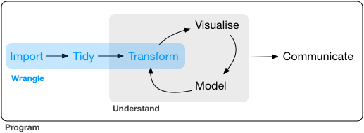
Here is a schematic taken from this book, that illustrates the typical data analysis workflow. In general, much of data science consists of wrangling data, or getting it in shape for visualization and analysis.
The core tidyverse set of packages includes:
- tidyr, for data tidying
- dplyr, for data transformation
- readr, for data import
- tibble, for tibbles, a re-imagining of data frames
- magrittr, for implementing the ‘pipe’ operator
- ggplot2, for data visualisation (the subject of the next module)
- purrr, for functional programming
- stringr, for strings
- forcats, for factors (categorical variables)
- lubridate, for dates
The following cheat sheets will be helpful in this module:
data ‘tidying’ data transformation working with dates and times
Learning goals
- Get more comfortable with tidyverse grammar (e.g., piping) and data structures to perform basic data manipulation tasks
- Use tidyr and dplyr data transformation ‘verbs’ to wrangle data
- Work with and parse dates using lubridate
Import sample data
The next few examples use meteorological data from Hungry Horse (HH) and Polson Kerr (PK) dams. You can download this data set by clicking here. Make sure you download this data set into your project directory!!
Let’s load this data into R!
#  Import and "tidy" your data  -----------------------------

# import meteorological data from Hungry Horse (HH) and Polson Kerr (PK) dams as tibble dataframe using readr
clim_data <- read_csv("MTMetStations.csv")

# quick look at the contents
clim_data
## # A tibble: 1,734 × 7
## Date PK.TMaxF PK.TMinF PK.PrcpIN HH.TMaxF HH.TMinF HH.PrcpIN
## <chr> <dbl> <dbl> <dbl> <dbl> <dbl> <dbl>
## 1 1/1/2013 27 19 0 26 22 0
## 2 1/2/2013 27 22 0 27 23 0
## 3 1/3/2013 23 14 0 25 21 0
## 4 1/4/2013 25 19 0 22 13 0
## 5 1/5/2013 29 20 0 24 13 0
## 6 1/6/2013 36 25 0 30 20 0.1
## 7 1/7/2013 35 30 0.16 35 22 0.23
## 8 1/8/2013 39 32 0.04 36 25 0.32
## 9 1/9/2013 44 31 0.07 39 30 0.1
## 10 1/10/2013 39 27 0.22 46 32 0.1
## # ℹ 1,724 more rows # display the last few lines of the data frame (often useful to check!)
tail(clim_data)## # A tibble: 6 × 7
## Date PK.TMaxF PK.TMinF PK.PrcpIN HH.TMaxF HH.TMinF HH.PrcpIN
## <chr> <dbl> <dbl> <dbl> <dbl> <dbl> <dbl>
## 1 9/25/2017 59 47 0.001 56 39 0
## 2 9/26/2017 66 47 0 58 43 0
## 3 9/27/2017 66 41 0 68 43 0
## 4 9/28/2017 67 39 0 66 43 0
## 5 9/29/2017 70 40 0 71 38 0
## 6 9/30/2017 62 47 0.06 71 38 0Making data tidy!
The tidyr package has several functions to help you get your
data into this format. The most important ones are
pivot_longer() and pivot_wider().
Use separate() to separate a single column into two
separate columns. unite() does the opposite
Let’s take a close look at the climate dataset and see if there’s anything we need to tidy up.
#  Use Tidyr verbs to make data 'tidy'

# look at clim_data -- is it in tidy format? What do we need to do to get it there?
head(clim_data)
## # A tibble: 6 × 7
## Date PK.TMaxF PK.TMinF PK.PrcpIN HH.TMaxF HH.TMinF HH.PrcpIN
## <chr> <dbl> <dbl> <dbl> <dbl> <dbl> <dbl>
## 1 1/1/2013 27 19 0 26 22 0
## 2 1/2/2013 27 22 0 27 23 0
## 3 1/3/2013 23 14 0 25 21 0
## 4 1/4/2013 25 19 0 22 13 0
## 5 1/5/2013 29 20 0 24 13 0
## 6 1/6/2013 36 25 0 30 20 0.1First of all, recall that tidy data should have have a single observation per row. In this case, each row represents observations taken from two different observatories: PK and HH. Ultimately, we want each row to represent a single date at a single station, one column to represent the station, and three columns to represent three different measurements: TMaxF, TMinF, and PrcpIN.
Our strategy will be the following:
- Use
pivot_longer()to make one row for every measurement at every station. - Use
separate()to separate station labels from climate variable labels. - Use
pivot_wider()to put all three measurements from each date/station into its own row.
The first step looks like this:
# step 1: pivot this data frame into long format:
#    we will create a new column called 'climvar_station', and all of the numeric precip and temp values into a column called 'value'.
clim_vars_longer <- clim_data %>% pivot_longer(
                           cols = !Date,
                           names_to = "climvar_station",
                           values_to = "value"
                    )

clim_vars_longer
## # A tibble: 10,404 × 3
## Date climvar_station value
## <chr> <chr> <dbl>
## 1 1/1/2013 PK.TMaxF 27
## 2 1/1/2013 PK.TMinF 19
## 3 1/1/2013 PK.PrcpIN 0
## 4 1/1/2013 HH.TMaxF 26
## 5 1/1/2013 HH.TMinF 22
## 6 1/1/2013 HH.PrcpIN 0
## 7 1/2/2013 PK.TMaxF 27
## 8 1/2/2013 PK.TMinF 22
## 9 1/2/2013 PK.PrcpIN 0
## 10 1/2/2013 HH.TMaxF 27
## # ℹ 10,394 more rowsIn the second step, we separate the station and climate variable labels into two different columns:
# step 2: separate the climvar_station column into two separate columns that identify the climate variable and the station
clim_vars_separate <- clim_vars_longer %>% separate(
                           col = climvar_station,
                           into = c("Station","climvar")
                      )

clim_vars_separate
## # A tibble: 10,404 × 4
## Date Station climvar value
## <chr> <chr> <chr> <dbl>
## 1 1/1/2013 PK TMaxF 27
## 2 1/1/2013 PK TMinF 19
## 3 1/1/2013 PK PrcpIN 0
## 4 1/1/2013 HH TMaxF 26
## 5 1/1/2013 HH TMinF 22
## 6 1/1/2013 HH PrcpIN 0
## 7 1/2/2013 PK TMaxF 27
## 8 1/2/2013 PK TMinF 22
## 9 1/2/2013 PK PrcpIN 0
## 10 1/2/2013 HH TMaxF 27
## # ℹ 10,394 more rowsFinally, let’s put climate measurements from a single station on the same row:
# step 3: pivot_wider distributes the clim_var column into separate columns, with the data values from the 'value' column

tidy_clim_data <- clim_vars_separate %>% pivot_wider(
                        names_from = climvar,
                        values_from = value
                  )

tidy_clim_data
## # A tibble: 3,468 × 5
## Date Station TMaxF TMinF PrcpIN
## <chr> <chr> <dbl> <dbl> <dbl>
## 1 1/1/2013 PK 27 19 0
## 2 1/1/2013 HH 26 22 0
## 3 1/2/2013 PK 27 22 0
## 4 1/2/2013 HH 27 23 0
## 5 1/3/2013 PK 23 14 0
## 6 1/3/2013 HH 25 21 0
## 7 1/4/2013 PK 25 19 0
## 8 1/4/2013 HH 22 13 0
## 9 1/5/2013 PK 29 20 0
## 10 1/5/2013 HH 24 13 0
## # ℹ 3,458 more rowsNote: we can do all of these tidying steps at once using the pipe operator:
# repeat above as single pipe series without creation of intermediate datasets

tidy_clim_data <- clim_data %>%
  pivot_longer(cols = !Date,
               names_to = "climvar_station",
               values_to = "value") %>%
  separate(col = climvar_station,
           into = c("Station","climvar")) %>%
  pivot_wider(names_from = climvar,
              values_from = value)

tidy_clim_data
## # A tibble: 3,468 × 5
## Date Station TMaxF TMinF PrcpIN
## <chr> <chr> <dbl> <dbl> <dbl>
## 1 1/1/2013 PK 27 19 0
## 2 1/1/2013 HH 26 22 0
## 3 1/2/2013 PK 27 22 0
## 4 1/2/2013 HH 27 23 0
## 5 1/3/2013 PK 23 14 0
## 6 1/3/2013 HH 25 21 0
## 7 1/4/2013 PK 25 19 0
## 8 1/4/2013 HH 22 13 0
## 9 1/5/2013 PK 29 20 0
## 10 1/5/2013 HH 24 13 0
## # ℹ 3,458 more rowsUsing dplyr – the data wrangling workhorse
dplyr is by far one of the most useful packages in all of the tidyverse as it allows you to quickly and easily summarize and manipulate your data once you have it in tidy form.
We have already worked with dplyr. The basic dplyr verbs include:
  * grouping data with *group_by()*
  * filtering rows with *filter()*
  * creating new variables with *mutate()*
  * summarizing with *summarize()*
  * selecting columns with *select()*
  * sorting columns by row with *arrange()*
# Use dplyr verbs to wrangle data ----------------------------
# example of simple data selection and summary using group_by, summarize, and mutate verbs
# take tidy_clim_data, then
# group data by station, then
# calculate summaries and put in columns with names mean.precip.in, mean.TMax.F, and mean.Tmin.F, then
# transform to metric and put in new columns mean.precip.in, mean.TMax.F, and mean.Tmin.F
station_mean1 <- tidy_clim_data %>%
group_by(Station) %>%
summarize(
mean.precip.in = mean(PrcpIN, na.rm=TRUE),
mean.TMax.F = mean(TMaxF, na.rm=TRUE),
mean.TMin.F = mean(TMinF, na.rm=TRUE)) %>%
mutate(
mean.precip.mm = mean.precip.in * 25.4,
mean.TMax.C = (mean.TMax.F - 32) * 5 / 9,
mean.TMin.C = (mean.TMin.F - 32) * 5 / 9
)
station_mean1## # A tibble: 2 × 7
## Station mean.precip.in mean.TMax.F mean.TMin.F mean.precip.mm mean.TMax.C
## <chr> <dbl> <dbl> <dbl> <dbl> <dbl>
## 1 HH 0.0972 56.0 36.3 2.47 13.3
## 2 PK 0.0442 57.8 36.5 1.12 14.3
## # ℹ 1 more variable: mean.TMin.C <dbl>There are several tricks that tidyverse provides that allow you to write as compact code as possible (avoiding re-typing the same code).
For example, the above code block involves doubling the formula for converting to celsius.
# using an even more compact form:

# take tidy_clim_data, then
# group data by station, then
# calculate summary (mean of all non-NA values) for numeric data only, then
# transform temp data (.) from F to C, then
# transform precip data (.) from in to mm


station_mean2 <- tidy_clim_data %>%
  group_by(Station) %>%
  summarize(across(where(is.numeric), mean, na.rm=TRUE)) %>%
  mutate(across(c("TMaxF", "TMinF"), ~(.-32)*(5/9)))   %>%
  rename_with(~gsub("F","C",.),starts_with("T")) %>%
  mutate(across(PrcpIN, ~.*25.4,.names="Prcp_mm")) %>%
  select(!PrcpIN)

station_mean2
## # A tibble: 2 × 4
## Station TMaxC TMinC Prcp_mm
## <chr> <dbl> <dbl> <dbl>
## 1 HH 13.3 2.36 2.47
## 2 PK 14.3 2.48 1.12Working with Dates with lubridate - Date from character string
Dates can be tricky to work with and we often want to eventually get
to the point that we can summarize our data by years, seasons, months,
or even day of the year. The lubridate package in R (also part
of the tidyverse) is very useful for creating and parsing dates for this
purpose. Date/time data often come as strings in a variety of
orders/formats. Lubridate is useful because it
automatically works out the date format once you specify the order of
the components. To do this, identify the order in which year, month, and
day appear in your dates, then arrange “y”, “m”, and “d” in the same
order. That gives you the name of the lubridate function that will parse
your date!
For example:
#  Using lubridate to format and create date data types -----------------

library(lubridate)

date_string <- ("2017-01-31")

# convert date string into date format by identifing the order in which
#   year, month, and day appear in your dates, then arrange "y", "m", and #   "d" in the same order. That gives you the name of the lubridate
#    function that will parse your date

ymd(date_string)
## [1] "2017-01-31"# note the different formats of the date_string and date_dtformat objects in the environment window.
# a variety of other formats/orders can also be accommodated. Note how each of these are reformatted to "2017-01-31" A timezone can be specified using tz=
mdy("January 31st, 2017")## [1] "2017-01-31"dmy("31-Jan-2017")## [1] "2017-01-31"ymd(20170131)## [1] "2017-01-31"ymd(20170131, tz = "UTC")## [1] "2017-01-31 UTC"# can also make a date from components.
# this is useful if you have columns for year, month,
# day in a dataframe
year<-2017
month<-1
day<-31
make_date(year, month, day)## [1] "2017-01-31"# times can be included as well. Note that unless otherwise specified, R assumes UTC time
ymd_hms("2017-01-31 20:11:59")## [1] "2017-01-31 20:11:59 UTC"mdy_hm("01/31/2017 08:01")## [1] "2017-01-31 08:01:00 UTC"# we can also have R tell us the current time or date
now()## [1] "2024-02-01 20:45:38 PST"today()## [1] "2024-02-01"Working with Dates with lubridate - Parsing Dates
Once dates are in date format, we can easily pull out their individual components like this:
#  Parsing dates with lubridate

datetime <- ymd_hms("2016-07-08 12:34:56")

# year
year(datetime)
## [1] 2016# month as numeric
month(datetime)## [1] 7# month as name
month(datetime, label = TRUE)## [1] Jul
## 12 Levels: Jan < Feb < Mar < Apr < May < Jun < Jul < Aug < Sep < ... < Dec# day of month
mday(datetime)## [1] 8# day of year (often incorrectly referred to as julian day)
yday(datetime)## [1] 190# day of week
wday(datetime)## [1] 6wday(datetime, label = TRUE, abbr = FALSE)## [1] Friday
## 7 Levels: Sunday < Monday < Tuesday < Wednesday < Thursday < ... < SaturdayWorking with Dates - Parsing Dates Example
We can use lubridate and dplyr to make new columns from a date for year, month, day of month, and day of year
first we convert the character string date into date format. Here we are naming the new column “Date”, so R will replace character string with date formatted dates
###  Using lubridate with dataframes and dplyr verbs

# going back to our tidy_clim_data dataset we see that
#   the date column is formatted as character, not date

head(tidy_clim_data)
## # A tibble: 6 × 5
## Date Station TMaxF TMinF PrcpIN
## <chr> <chr> <dbl> <dbl> <dbl>
## 1 1/1/2013 PK 27 19 0
## 2 1/1/2013 HH 26 22 0
## 3 1/2/2013 PK 27 22 0
## 4 1/2/2013 HH 27 23 0
## 5 1/3/2013 PK 23 14 0
## 6 1/3/2013 HH 25 21 0# change format of date column
tidy_clim_data <- tidy_clim_data %>%
mutate(Date = mdy(Date))
tidy_clim_data## # A tibble: 3,468 × 5
## Date Station TMaxF TMinF PrcpIN
## <date> <chr> <dbl> <dbl> <dbl>
## 1 2013-01-01 PK 27 19 0
## 2 2013-01-01 HH 26 22 0
## 3 2013-01-02 PK 27 22 0
## 4 2013-01-02 HH 27 23 0
## 5 2013-01-03 PK 23 14 0
## 6 2013-01-03 HH 25 21 0
## 7 2013-01-04 PK 25 19 0
## 8 2013-01-04 HH 22 13 0
## 9 2013-01-05 PK 29 20 0
## 10 2013-01-05 HH 24 13 0
## # ℹ 3,458 more rowsNow we can use mutate to create individual columns for the date components
# parse date into year, month, day, and day of year columns
tidy_clim_data <- tidy_clim_data %>%
  mutate(
    Year = year(Date),
    Month = month(Date),
    Day = mday(Date),
    Yday = yday(Date)
  )

tidy_clim_data
## # A tibble: 3,468 × 9
## Date Station TMaxF TMinF PrcpIN Year Month Day Yday
## <date> <chr> <dbl> <dbl> <dbl> <dbl> <dbl> <int> <dbl>
## 1 2013-01-01 PK 27 19 0 2013 1 1 1
## 2 2013-01-01 HH 26 22 0 2013 1 1 1
## 3 2013-01-02 PK 27 22 0 2013 1 2 2
## 4 2013-01-02 HH 27 23 0 2013 1 2 2
## 5 2013-01-03 PK 23 14 0 2013 1 3 3
## 6 2013-01-03 HH 25 21 0 2013 1 3 3
## 7 2013-01-04 PK 25 19 0 2013 1 4 4
## 8 2013-01-04 HH 22 13 0 2013 1 4 4
## 9 2013-01-05 PK 29 20 0 2013 1 5 5
## 10 2013-01-05 HH 24 13 0 2013 1 5 5
## # ℹ 3,458 more rows# calculate total annual precipitation by station and year
annual_sum_precip_by_station <- tidy_clim_data %>%
group_by(Station, Year) %>%
summarise(PrecipSum = sum(PrcpIN))
annual_sum_precip_by_station ## # A tibble: 10 × 3
## # Groups: Station [2]
## Station Year PrecipSum
## <chr> <dbl> <dbl>
## 1 HH 2013 29.8
## 2 HH 2014 40.8
## 3 HH 2015 25.7
## 4 HH 2016 47.0
## 5 HH 2017 25.1
## 6 PK 2013 14.7
## 7 PK 2014 19.9
## 8 PK 2015 12.6
## 9 PK 2016 17.7
## 10 PK 2017 11.8Challenge Exercises
- Try to put tidyr’s built-in
relig_incomedataset into a tidier format. This dataset stores counts based on a survey which (among other things) asked people about their religion and annual income:
Your final result should look like this:
## # A tibble: 180 × 3
##    religion Income             count
##    <chr>    <chr>              <dbl>
##  1 Agnostic <$10k                 27
##  2 Agnostic $10-20k               34
##  3 Agnostic $20-30k               60
##  4 Agnostic $30-40k               81
##  5 Agnostic $40-50k               76
##  6 Agnostic $50-75k              137
##  7 Agnostic $75-100k             122
##  8 Agnostic $100-150k            109
##  9 Agnostic >150k                 84
## 10 Agnostic Don't know/refused    96
## # ℹ 170 more rows
Use the dplyr verbs and the tidy_clim_data dataset you created above to calculate monthly average Tmin and Tmax for each station
Using lubridate, make a date object out of a character string of your birthday (you can use a fake birthday if you want!) and find the day of week it occurred on. Note, you can use the ‘wday’ function in lubridate to extract the day of the week (1 is sunday).
# CHALLENGE EXERCISES   -------------------------------------

# 1. Try to put tidyr's built-in `relig_income` dataset into a tidier format.
#      This dataset stores counts based on a survey which (among other things)
#      asked people about their religion and annual income:

# 2. Use the dplyr verbs and the tidy_clim_data dataset you created above
#       to calculate monthly average Tmin and Tmax for each station (in Fahrenheit is okay)

# 3. Using lubridate, make a date object out of a character string of your
#        birthday and find the day of week it occurred on. Note, you
#        can use the 'wday' function in lubridate to extract the day of the
#         week (1 is sunday).