September 2017

9/21/2017

We discussed Zach Marion’s Bayesian model for partitioning diversity.

9/14/2017

Initial planning meeting for Fall 2017 semester.

February 2017

2/28/2017

Mostly we discussed putting together a Google spreadsheet as a one-stop shop for students to find quantitative course offerings on campus (click here). Next week we will discuss Justin’s red-tailed hawk data set.

2/21/2017

Jessi Brown led a discussion/tutorial about parallelizing analyses in R using the ‘parallel’ package. The code will be made available on this website soon. Next week we will continue this discussion and discuss how to port this code for a Windows OS.

2/14/2017

First meeting of the semester (after a fashionable delay). Introduction and planning for the spring semester. Sounds like there is interest in workshop-type sessions focused on particular topics of interest. Among the topics discussed were parallel computing in R, SQL databases, use of “the grid”, ordination, and GitHub. For next week: parallel computing in R, led by Stats Chats co-leader Jessi Brown. We also discussed the possibility of hosting a list of quantitative course offerings at UNR, along with a brief description of the target audience for each class.

December 2016

12/6/2016

Discussion topic: SECR in JAGS for woodrats Discussion leader: Kevin Shoemaker and Elizabeth Hunter We will discuss a model for estimating survival and movement propensity for two species of woodrats within a hybrid zone. We are using a modified CJS model in a spatially-explicit capture-recapture (secr) framework.

model{
    ############
    #PRIORS
    #Survival
    phi0 ~ dunif(0, 1)      #mean survival rate
    logit.phi <- log(phi0/(1-phi0)) #survival on logit scale

    juvEff ~ dunif(-4,4)            #beta term for juvenile effect on survival
    maleEff ~ dunif(-4,4)           #beta term for sex effect on survival
    FuEff ~ dunif(-4,4)         #beta terms for effect of genotype on survival
    MaEff ~ dunif(-4,4)
    bcFuEff ~ dunif(-4,4)
    bcMaEff ~ dunif(-4,4)

    male.prob ~ dunif(0,1)   # probability of being male (account for unknown sex)
    Fu.prob ~ dunif(0,1)     # probability of being a given genotype (account for unknown genotype)
    Ma.prob ~ dunif(0,1)
    bcFu.prob ~ dunif(0,1)
    bcMa.prob ~ dunif(0,1)

    #Some individuals are not sexed or genotyped, so need priors for those missing data
    for(i in 1:n.ind){
        isMale[i] ~ dbern(male.prob)
        isFu[i] ~ dbern(Fu.prob)
        isMa[i] ~ dbern(Ma.prob)
        isbcFu[i] ~ dbern(bcFu.prob)
        isbcMa[i] ~ dbern(bcMa.prob)
    }

    #Detection    
    lambda0.base ~ dunif(0.001, 0.5)    # mean times resident indiv captured at its given house per independent survey event
    #logit.lambda0.base <- log(lambda0.base/(1-lambda0.base))       
    sigma ~ dunif(0, 500)   # drop off in detection with distance   
    sigma2 <- pow(sigma,2)

    #Movement among houses
    p.move.male ~ dunif(0, 0.3)
    p.move.female ~ dunif(0, 0.3)

    ###########
    #HOUSE MODEL

    for (i in 1:n.ind){
            myHouse[i,firsts[i]] <- firstHouse[i]  #~ dcat(firstHouseProb[i,])
            p.move[i] <- isMale[i] * p.move.male + (1-isMale[i])*p.move.female
        for(t in (firsts[i]+1):n.periods){
            transitionHouse[i,t] <- pow(p.move[i], period[t-1])  #Probability of transitioning to a new house
            newHouseCand_unif[i,t] ~ dunif(0,n.houses)    # this could be turned into a distance kernel using the ones trick?
            newHouseCand_cat[i,t] <- trunc(newHouseCand_unif[i,t]+1) #~ dcat(houseprob[])  #
            move[i,t] ~ dbern(transitionHouse[i,t])     #latent variable: did it move to a new activity center?
            myHouse[i,t] <-  move[i,t]*newHouseCand_cat[i,t] + (1-move[i,t])*myHouse[i,t-1]     # which house does it live in now???  newHouse[i,t]
        }
    }

    ############
    #OBSERVATION MODEL

    for(i in 1:n.ind){
        for(t in (firsts[i]+1):n.periods){
            #Loop only through traps near to myHouse (<200m away) that are open within a period 
            for(r in 1:nearopen.num[firstHouse[i],t]){                
                    lambda[i,t,nearopen[t,r,firstHouse[i]]] <- lambda0.base * exp(-1*(D2[myHouse[i,t],nearopen[t,r,firstHouse[i]]])/(2*sigma2 )) * alive[i,t]    #total exposure as function of distance
                    ind.trap.per[i,nearopen[t,r,firstHouse[i]],t] ~ dbin(lambda[i,t,nearopen[t,r,firstHouse[i]]],eff.per[nearopen[t,r,firstHouse[i]],t])
            }
        }
    }

    ############
    #SURVIVAL MODEL

    for(i in 1:n.ind){
            for(t in 1:(firsts[i]-1)){
            alive[i,t] ~ dbern(1)
            }
    }

    for(i in 1:n.ind){
        for(t in 1:(n.periods-1)){
            mu.phi[i,t] <- logit.phi + maleEff*isMale[i] + juvEff*isJuv[i,t] + FuEff*isFu[i] + MaEff*isMa[i] + bcFuEff*isbcFu[i] + bcMaEff*isbcMa[i]
                #EAH: changed mu.phi to be period specific instead of just [i]
            logit(phi[i,t]) <- mu.phi[i,t]   # expected survival rate for this individual at this time on the basis of covariates
        }
    }


    #Latent variable: living or dead
    for(i in 1:n.ind){
        alive[i,firsts[i]] ~ dbern(1)       #At first capture, individual is alive
        for(t in (firsts[i]+1):n.periods){
            transition[i,t] <- pow(phi[i,t-1], period[t-1])  #Probability of transitioning to this period (based on period duration)
            mualive[i,t] <- alive[i,(t-1)] * transition[i,t]    #probability of each ind being alive after transitioning
            alive[i,t] ~ dbern(mualive[i,t])        #latent variable: is it still alive?
        }
    }

} #END MODEL

November 2016

11/29/2016

Discussion topic: Mixed effects modeling. Although Pinhiero and Bates suggest that LRT is appropriate for mixed effects models, we are still unsure how to compute the degrees of freedom for the Chi-squared distribution that describes the null hypothesis. We are also wondering exactly why it is not recommended to use information criteria to compare models with different random effects structures. Paul mentioned the possibility of generating null distributions for such questions and seeing how well they match with the Chi-squared distribution recommended by pinhiero and bates.. Phillip mentioned that Ken Burnham “solved” this issue by using the trace of the “G-matrix” to approximate the number of free parameters in the model.

Here are some links with good guidance!!

Link1
Link2

11/22/2016

Discussion leader: Jessi Brown, Chris Vennum We discussed what you can do with mixed models once you have fitted them using something like “lmer” from the “lme4” package in R. In partucular, we discussed how to use R to bootstrap predictions from mixed effects models and whether confidence intervals from lmer compared favorably with those from a Bayesian modeling approach in JAGS.

11/15/2016

Leader: Chris Vennum We continued our discussion of linear mixed models- in particular, we discussed (1) strategies for evaluating the normality of residuals if the random effect terms do most of the explaining, and (2) whether parameter estimation breaks down if some or all predictor variables are perfectly correlated with a “group” variable (all sampling units within a group share the same covariate value). For the latter case, using a simulation (below), Thomas Riecke demonstrated that the REML algorithm in “lmer” was able to estimate fixed effects terms appropriately.

#########################################################################
# group number, cluster size
#########################################################################
groups <- 50
cluster <- 5

#########################################################################
# generate random groups
#########################################################################
random <- seq(1,groups,1)                               # 100 random groups
data <- data.frame(rep(random, each = cluster))            # build a data.frame with 10 observations per cluster

#########################################################################
# generate 100 covariate values
#########################################################################
x <- rnorm(groups, 0, 2); hist(x)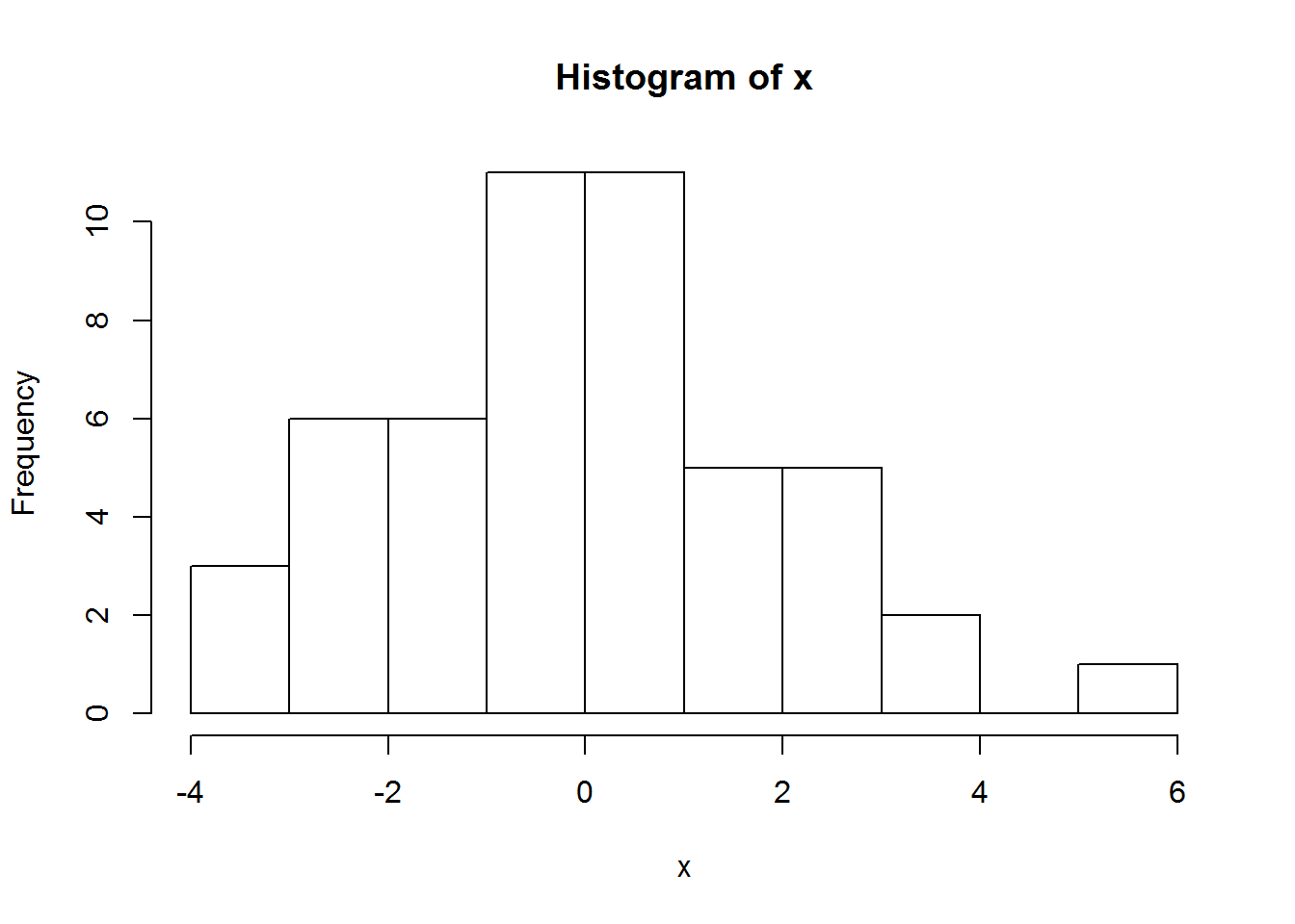

data[,2] <- NA

#########################################################################
# assign covariate values to groups... all the same
#########################################################################
for (i in 1:nrow(data)){
  data[i,2] <- x[data[i,1]]
}

#########################################################################
# generate data with noise
#########################################################################
alpha <- 5
beta <- 1
data[,3] <- alpha + data[,2] * beta + rnorm(groups * cluster, 0, 3) 

par(family = 'serif', mar = c(5.1,5.1,2.1,2.1))
plot(data[,3] ~ data[,2], ylab = 'Response', xlab = 'Covariate', cex.lab = 2)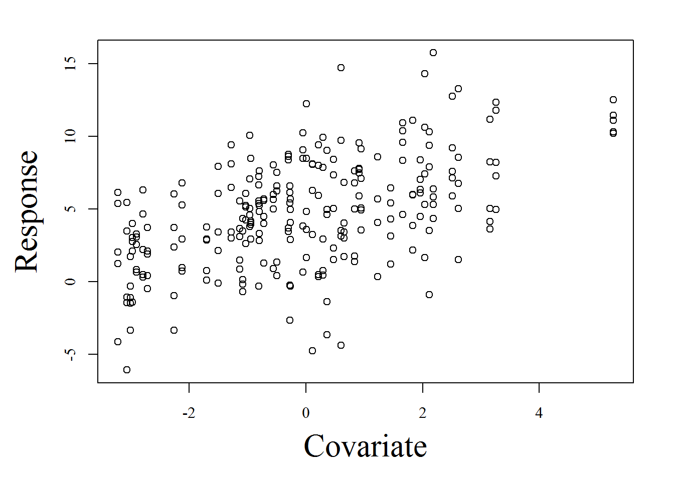

#########################################################################
# assign less ridiculous column names
#########################################################################
colnames(data) <- c('group', 'covariate', 'response')

library(lme4)
summary(lmer(response ~ covariate + (1|group), data = data))

## Linear mixed model fit by REML ['lmerMod']
## Formula: response ~ covariate + (1 | group)
##    Data: data
## 
## REML criterion at convergence: 1294.7
## 
## Scaled residuals: 
##      Min       1Q   Median       3Q      Max 
## -3.05573 -0.64367  0.01365  0.63005  2.89404 
## 
## Random effects:
##  Groups   Name        Variance Std.Dev.
##  group    (Intercept)  0.00    0.000   
##  Residual             10.31    3.211   
## Number of obs: 250, groups:  group, 50
## 
## Fixed effects:
##             Estimate Std. Error t value
## (Intercept)   4.8051     0.2031  23.655
## covariate     1.0443     0.1077   9.699
## 
## Correlation of Fixed Effects:
##           (Intr)
## covariate 0.025

11/8/2016

Since no one came with questions, we discussed mixed models. Several ‘stats chats’ participants over the last year have raised the question of how to determine the ‘significance’ of random effects, and how to decide whether to keep or remove specific random effects from a (generalized) linear mixed model. We discussed the possibility of running bootstrap tests in R to determine whether more variance is explained by the random effect than would be predicted on the basis of random chance. Paul raised the question of whether you can test for abnormal random effects distributions- e.g., bimodal distributions. We will continue this discussion next week…

11/1/2016

Since no one came with questions, we discussed the quantitative curriculum at UNR for graduate students and undergraduates. We started out by wondering aloud if coding and quantitive analysis could be embedded in the curriculum so that students had more exposure to these tools in many different contexts. Some key points of our discussion:

We need to reach out to Tom Parchman in Biology to discuss whether his existing class could serve as a basic introduction to programming for grad students.
Students need more consistent exposure to coding, stats, and mathematics (e.g., calc, linear algebra)
Bootcamps can serve a useful purpose: e.g., programming in R and python, Calculus review, linear algebra review, probability review
Grad students are in need of more 700-level courses. Several grad students would like to pursue a “crash course” in basic mathematical concepts, potentially following Otto and Day, and potentially to be offered in Fall 2017.

Topics

Stats Chats

September 27, 2017

Other future topics?