Week 10: Model Comparison and Regularization
NRES 746
Oct. 26-28, 2026
R code from this page is also in the companion script. Packages: emdbook, MASS, glmnet, cmdstanr, loo.
This material follows Bolker, Ecological Models and Data in R, section 6.6 (pp. 267-290).
Likelihood ratio tests, AIC, and regularization
How do we compare models that differ in complexity? This part covers the most rigorous test (predicting new data), two shortcuts that need only one fit (the likelihood ratio test and AIC), and regularization, which keeps every covariate in a single model and shrinks the coefficients toward 0.
1. Big picture
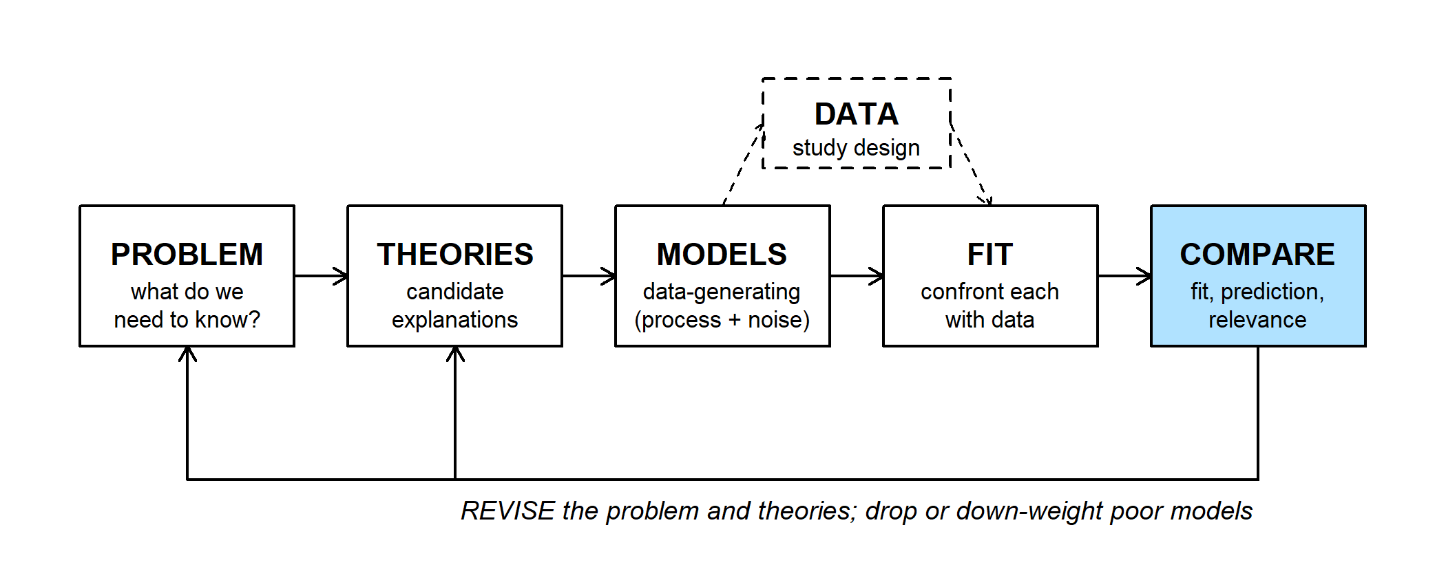
The FIT step gives estimates and their uncertainty for one model at a time. COMPARE weighs models against each other. It has three parts:
- Does the model fit the data at all?
- Does it beat its rivals, including a null model, and predict new data?
- Is it relevant to the problem we started with? (A judgment, not a statistic.)
Here we focus on part 2, comparing models fit to the same data. This includes:
- Null-model tests: is there evidence that a model (a theory) outperforms an uninteresting one?
- Model selection: which of several alternative models is best supported by the data?
- Multimodel inference: when several models have some support, base predictions and inferences on all of them.
Adding parameters always improves the fit to the data in hand (see the WOD), so in-sample fit can't answer these questions. The most rigorous test is how well a model predicts new data from the same process:
- Validation: fit the model to one data set and score its predictions on data it never saw, ideally collected separately.
- Cross-validation: without new data, hold out part of the data, fit to the rest, score the held-out part, and rotate. This means fitting the model many times. (More on this later in the course.)
Because cross-validation takes many refits, we often rely on shortcuts that use a single fit to all the data:
- LRT: does a bigger (nested) model fit better than chance alone would explain?
- AIC: estimates how well a model would predict new data. In large samples it ranks models about the same way leave-one-out cross-validation does.
Ridge regression and the lasso take a third route: fit one large model and penalize the size of its coefficients, usually choosing the penalty strength by cross-validation.
Models that pass these tests are corroborated, not proven.
2. WOD: bias-variance tradeoff
The WOD (a short warm-up exercise at the start of class) gave seven measurements of seedling height and soil moisture, and two models: a straight line and a curve through every point. Both models were used to predict height at 19% moisture, where there were no data.
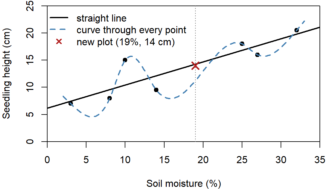
- Sum of squared residuals: line 35.2, curve 0.
- The new plot measured 14 cm. The line predicted 14.3; this curve predicted 11.2.
A perfect fit to seven points says little about prediction. Suppose we repeated the study many times with new seedlings from the same process, refitting both models each time:
- A very flexible model fits the noise along with the signal. Its predictions are about right on average (low bias) but swing widely from one sample to the next (high variance).
- A very simple model, such as a constant mean height, gives nearly the same prediction from every sample, but it misses a real trend, so it is consistently wrong (high bias, low variance).
Prediction error on new data includes both. More complexity lowers bias but raises variance, so the best predictive model lies somewhere between the extremes.
In the figure below, the study is repeated 20 times. Each sample uses the WOD's moisture values, with heights simulated from the red line plus random noise.
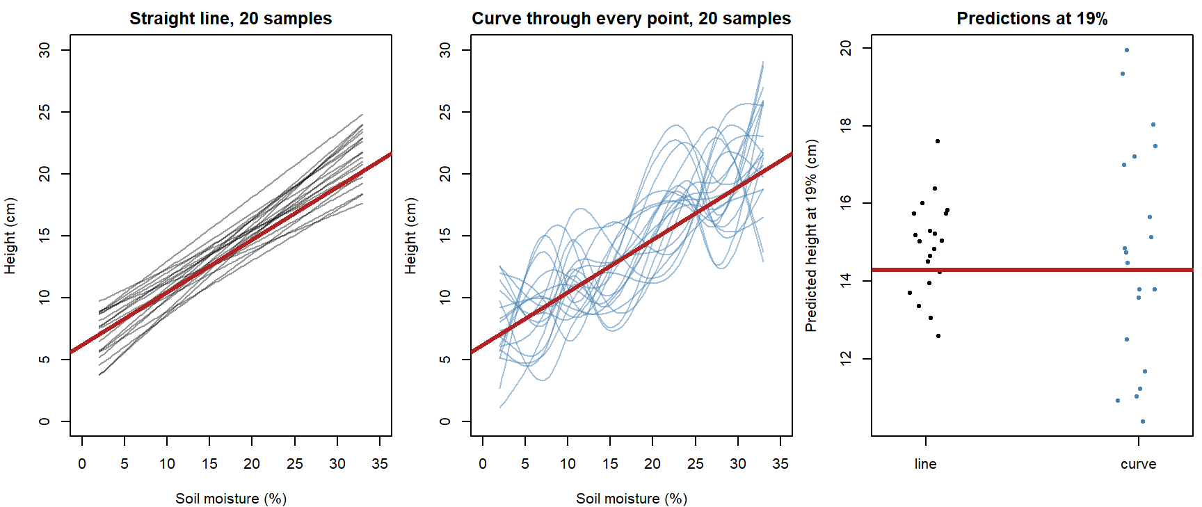
Both models center near the true height at 19% (red line), but the curve's predictions vary more than twice as much (SD 2.9 cm vs. 1.2 cm for the line).
3. Likelihood ratio test
Bolker's balsam fir data (section 6.6): cone counts on 242 trees, some at "wave" sites (where stands regenerate in waves) and some not. Model: \(\text{cones} \sim \text{NegBin}(\mu = a\,\text{DBH}^b, k)\). Do wave sites differ?
- Full model: separate \(a\), \(b\), \(k\) for wave and non-wave sites (6 parameters).
- Reduced model: one \(a\), \(b\), \(k\) for all trees (3 parameters).
The likelihood ratio test is the oldest shortcut. It applies to nested models, where the reduced model is the full model with some parameters fixed (often at 0). Here the reduced model fixes three: wave and non-wave sites share \(a\), \(b\), and \(k\).
Since the full model always fits at least as well, the real question is whether it fits better than extra parameters fitting pure noise would. If the reduced model is true, then in large samples the deviance
\[D = 2(\text{NLL}_{\text{reduced}} - \text{NLL}_{\text{full}})\]
follows a \(\chi^2_r\) distribution, where \(r\) is the number of fixed parameters (Wilks' theorem).
The test:
- Fit both models by maximum likelihood and record each minimum NLL.
- Compute \(D\). It is never negative, since the full model fits at least as well.
- Compare \(D\) with the 95% quantile of \(\chi^2_r\) (
qchisq(0.95, r)). - If \(D\) exceeds it (\(p < 0.05\)), the extra parameters improve the fit more than fitting noise usually would: evidence for the full model. Otherwise keep the reduced model, following the principle of parsimony.
The 1.92 cutoff for likelihood-based confidence intervals comes from the same result with \(r = 1\): \(\chi^2_1\)'s 95% quantile is 3.84, and \(3.84/2 = 1.92\) on the NLL scale.
library(emdbook)
fir <- na.omit(FirDBHFec[, c("TOTCONES", "DBH", "WAVE_NON")])   # balsam fir, 242 trees
fir$TOTCONES <- round(fir$TOTCONES)
wave <- as.numeric(fir$WAVE_NON)   # 1 = non-wave, 2 = wave

plot(TOTCONES ~ DBH, data = fir, col = wave, pch = 19,
     xlab = "DBH (cm)", ylab = "Total cones")
legend("topleft", c("non-wave", "wave"), col = 1:2, pch = 19, bty = "n")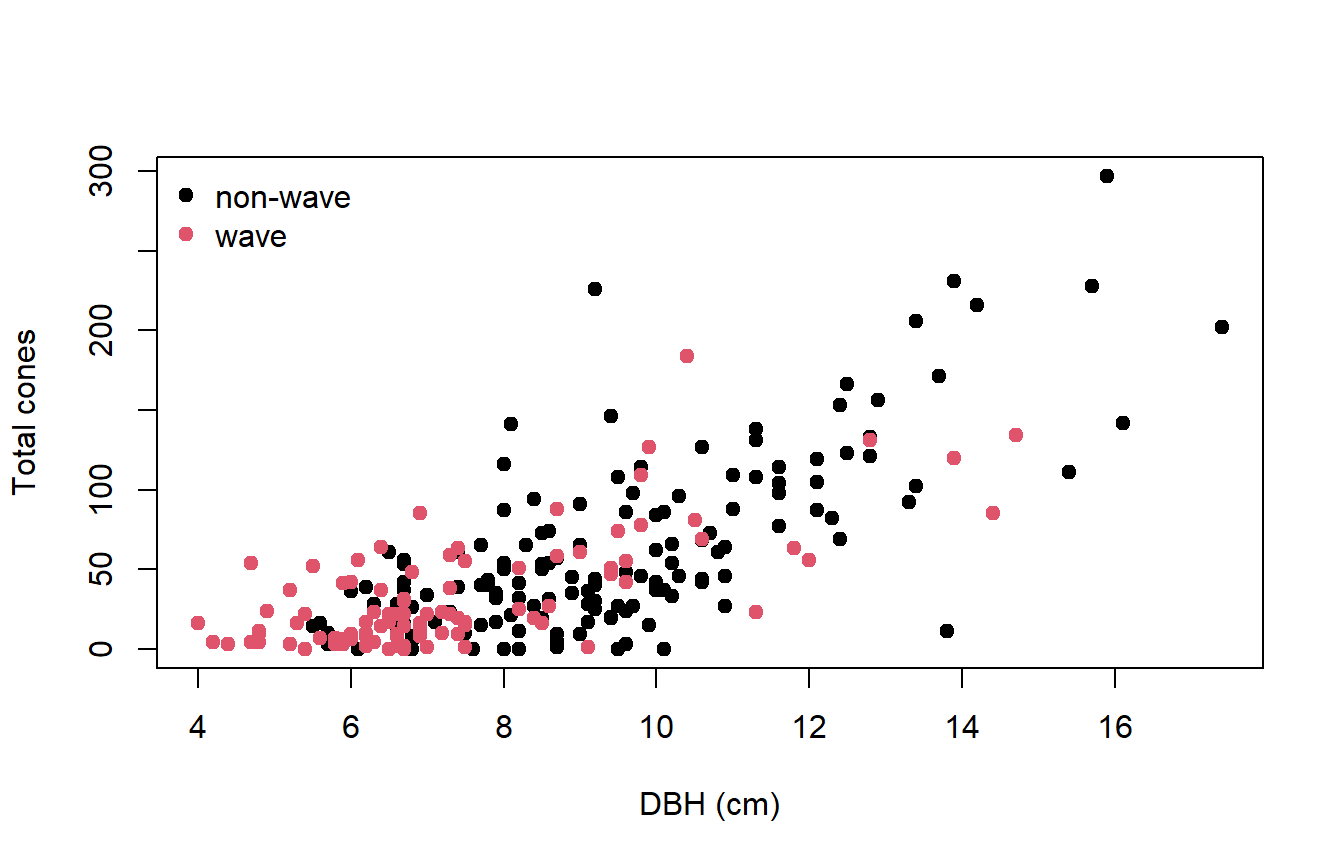
# cones ~ NegBin(mu = a * DBH^b, size = k); a, b, k can be vectors (one value per tree)
nll_nb <- function(a, b, k) {
  -sum(dnbinom(fir$TOTCONES, mu = a * fir$DBH^b, size = k, log = TRUE))
}

# full model: separate a, b, k for wave and non-wave sites (6 parameters)
nll_full <- function(p) nll_nb(p[1:2][wave], p[3:4][wave], p[5:6][wave])
# no-wave model: one a, b, k for all trees (3 parameters)
nll_nowave <- function(p) nll_nb(p[1], p[2], p[3])

# Nelder-Mead to get close, then BFGS to polish
fit_model <- function(nll, start) {
  fit <- optim(start, nll, control = list(maxit = 10000))
  optim(fit$par, nll, method = "BFGS", control = list(maxit = 10000))
}
fit_full <- fit_model(nll_full, c(1, 1, 2, 2, 1, 1))
fit_nowave <- fit_model(nll_nowave, c(1, 2, 1))
c(full = fit_full$value, nowave = fit_nowave$value)   # min NLL
## full nowave
## 1135.011 1136.015# deviance = 2 * (NLL_reduced - NLL_full) ~ chi-square, df = difference in parameters
deviance <- 2 * (fit_nowave$value - fit_full$value)
deviance## [1] 2.009181qchisq(0.95, df = 3) # critical value## [1] 7.814728pchisq(deviance, df = 3, lower.tail = FALSE) # p-value## [1] 0.5705034curve(dchisq(x, df = 3), 0, 12, lwd = 2, xlab = "Deviance", ylab = "Density",
main = "Deviance under the reduced model (df = 3)")
abline(v = qchisq(0.95, 3), lty = 2)
abline(v = deviance, col = "red", lwd = 3)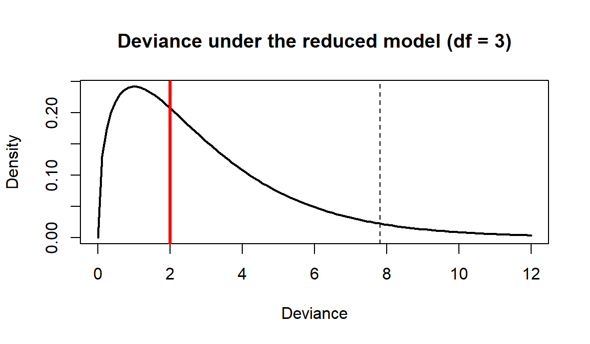
With \(D = 2.01\), well below the cutoff, we keep the no-wave model.
# Poisson, no wave effect (2 parameters)
nll_pois <- function(p) -sum(dpois(fir$TOTCONES, p[1] * fir$DBH^p[2], log = TRUE))
fit_pois <- fit_model(nll_pois, c(1, 2))
2 * (fit_pois$value - fit_nowave$value)
## [1] 4051.633Question: Is the Poisson model nested in the negative binomial? Can we use an LRT here?
Keeping the reduced model doesn't show that wave and non-wave trees are alike. It shows that these 242 trees can't distinguish them.
4. AIC
\[\text{AIC} = -2\log\mathcal{L}(\hat\theta) + 2k\]
AIC can rank any set of models fit to the same response data, nested or not. The \(2k\) term estimates how much the in-sample fit overstates the fit to new data (the problem in the WOD). The AIC penalty handout shows where it comes from.
- \(\Delta_i = \text{AIC}_i - \text{AIC}_{\min}\)
- Akaike weights: \(w_i = e^{-\Delta_i/2} / \sum_j e^{-\Delta_j/2}\)
- AICc adds a small-sample correction; BIC uses \(k \log n\) in place of \(2k\) (a harsher penalty).
# two intermediate models: wave changes only a and k (5 parameters), or only b (4)
nll_constb <- function(p) nll_nb(p[1:2][wave], p[3], p[4:5][wave])
nll_constak <- function(p) nll_nb(p[1], p[2:3][wave], p[4])
fit_constb <- fit_model(nll_constb, c(1, 1, 2, 1, 1))
fit_constak <- fit_model(nll_constak, c(1, 2, 2, 1))

fits <- list(full = fit_full, const_b = fit_constb, const_ak = fit_constak,
             no_wave = fit_nowave, poisson = fit_pois)
n <- nrow(fir)
aic_tab <- data.frame(model = names(fits),
                      k = sapply(fits, function(f) length(f$par)),
                      logLik = sapply(fits, function(f) -f$value))     # log L = -NLL
aic_tab$AIC <- -2 * aic_tab$logLik + 2 * aic_tab$k              # -2 log L + 2k
aic_tab$dAIC <- aic_tab$AIC - min(aic_tab$AIC)
aic_tab$weight <- exp(-aic_tab$dAIC / 2) / sum(exp(-aic_tab$dAIC / 2))
aic_tab$AICc <- aic_tab$AIC + 2 * aic_tab$k * (aic_tab$k + 1) / (n - aic_tab$k - 1)
aic_tab$BIC <- -2 * aic_tab$logLik + log(n) * aic_tab$k         # -2 log L + k log(n)
aic_tab <- aic_tab[order(aic_tab$AIC), ]
rownames(aic_tab) <- NULL| model | k | logLik | AIC | dAIC | weight | AICc | BIC |
|---|---|---|---|---|---|---|---|
| no_wave | 3 | -1136.02 | 2278.03 | 0.00 | 0.52 | 2278.13 | 2288.50 |
| const_ak | 4 | -1135.76 | 2279.52 | 1.48 | 0.25 | 2279.68 | 2293.47 |
| const_b | 5 | -1135.13 | 2280.27 | 2.24 | 0.17 | 2280.52 | 2297.71 |
| full | 6 | -1135.01 | 2282.02 | 3.99 | 0.07 | 2282.38 | 2302.95 |
| poisson | 2 | -3161.83 | 6327.66 | 4049.63 | 0.00 | 6327.71 | 6334.64 |
Question: The no-wave model has weight 0.52. Is there a 52% chance it's the true model?
Look at const_ak. It has one more parameter than the no-wave model and a log likelihood only 0.26 higher, yet it is just 1.48 AIC units behind. A useless parameter costs at most 2 AIC units, so being within 2 of the best model isn't evidence of support (Arnold 2010, J. Wildl. Manage. 74: 1175-1178).
5. Regularization: ridge and LASSO
Example: brown creepers. Counts at 50 point-count stations, with 10 standardized habitat covariates. These data are simulated, so we know the truth: only big trees, snags, and road distance matter.
Ten covariates give \(2^{10} = 1024\) possible subsets. Instead of searching them all, we can keep all 10 and penalize the size of the coefficients:
\[\text{ridge: } \text{NLL}(\beta) + \lambda\sum_j \beta_j^2 \qquad\qquad \text{lasso: } \text{NLL}(\beta) + \lambda\sum_j |\beta_j|\]
AIC charges for each parameter; these penalties grow with the size of the coefficients. One \(\lambda\) applies to every coefficient, so the covariates are standardized first. The lasso penalty has a corner at 0 that can set coefficients to exactly 0 (try the slider in Prices and budgets).
A penalty also makes the search simpler. Instead of comparing 1024 unordered models, we turn one dial: as \(\lambda\) falls from large to 0, the fit moves from the intercept alone to the full MLE, and cross-validation only has to choose a point along that path. The path passes through only a few of the 1024 subsets, in an order set by the data, so it can miss the best one. In exchange, its estimates are shrunk, and tuning one number overfits the held-out data less than picking a winner from a thousand models.
library(MASS)
library(glmnet)

# brown creeper counts at 50 point-count stations, 10 standardized habitat covariates.
# Simulated, so we know the truth: only big_trees, snags, and road_dist matter.
covars <- c("canopy", "big_trees", "snags", "shrub", "elev", "slope",
            "north", "road_dist", "stream_dist", "grazing")
beta_true <- c(0, 0.5, 0.4, 0, 0, 0, 0, 0.3, 0, 0)
cov_mat <- diag(10)
cov_mat[1, 2] <- cov_mat[2, 1] <- 0.6    # canopy ~ big trees
cov_mat[1, 4] <- cov_mat[4, 1] <- -0.4   # canopy ~ shrub
cov_mat[5, 6] <- cov_mat[6, 5] <- 0.5    # elevation ~ slope
set.seed(19)
X <- mvrnorm(50, rep(0, 10), cov_mat)
colnames(X) <- covars
creepers <- rpois(50, exp(log(2) + X %*% beta_true))   # log(mu) = log(2) + X beta

# ordinary MLE with every covariate: no estimate is exactly 0
fit_glm <- glm(creepers ~ X, family = poisson)
round(coef(fit_glm)[-1], 2)
## Xcanopy Xbig_trees Xsnags Xshrub Xelev Xslope
## -0.06 0.67 0.56 -0.06 0.11 -0.08
## Xnorth Xroad_dist Xstream_dist Xgrazing
## 0.22 0.37 -0.07 -0.03# all 2^10 = 1024 subsets, ranked by AIC
subsets <- expand.grid(rep(list(c(FALSE, TRUE)), 10))
subset_aic <- apply(subsets, 1, function(use) {
if (!any(use)) return(AIC(glm(creepers ~ 1, family = poisson)))
AIC(glm(creepers ~ X[, use, drop = FALSE], family = poisson))
})
covars[unlist(subsets[which.min(subset_aic), ])] # best subset## [1] "big_trees" "snags" "north" "road_dist"sum(subset_aic - min(subset_aic) < 2) # models within 2 AIC units## [1] 8# AIC table of the top models: k counts the intercept
subset_tab <- data.frame(
model = apply(subsets, 1, function(use) {
if (!any(use)) "(intercept only)" else paste(covars[use], collapse = " + ")
}),
k = rowSums(subsets) + 1,
AIC = subset_aic)
subset_tab$logLik <- (2 * subset_tab$k - subset_tab$AIC) / 2 # AIC = -2 log L + 2k
subset_tab <- subset_tab[c("model", "k", "logLik", "AIC")]
subset_tab$dAIC <- subset_tab$AIC - min(subset_tab$AIC)
subset_tab$weight <- exp(-subset_tab$dAIC / 2) / sum(exp(-subset_tab$dAIC / 2))
subset_tab <- subset_tab[order(subset_tab$AIC), ]
rownames(subset_tab) <- NULL| model | k | logLik | AIC | dAIC | weight |
|---|---|---|---|---|---|
| big_trees + snags + north + road_dist | 5 | -64.70 | 139.40 | 0.00 | 0.08 |
| big_trees + snags + road_dist | 4 | -66.13 | 140.25 | 0.86 | 0.05 |
| big_trees + snags + north + road_dist + stream_dist | 6 | -64.56 | 141.12 | 1.72 | 0.03 |
| big_trees + snags + elev + north + road_dist | 6 | -64.58 | 141.15 | 1.75 | 0.03 |
| big_trees + snags + slope + north + road_dist | 6 | -64.68 | 141.35 | 1.95 | 0.03 |
| big_trees + snags + shrub + north + road_dist | 6 | -64.68 | 141.36 | 1.96 | 0.03 |
| canopy + big_trees + snags + north + road_dist | 6 | -64.69 | 141.38 | 1.98 | 0.03 |
| big_trees + snags + north + road_dist + grazing | 6 | -64.70 | 141.39 | 1.99 | 0.03 |
| big_trees + snags + road_dist + stream_dist | 5 | -65.82 | 141.63 | 2.23 | 0.03 |
| big_trees + snags + road_dist + grazing | 5 | -65.95 | 141.89 | 2.49 | 0.02 |
Question: Which covariates show up in nearly every top model? Which come and go?
# penalized NLL: NLL(beta) + lambda * sum(beta^2) (ridge) or lambda * sum(|beta|) (lasso)
fit_ridge <- glmnet(X, creepers, family = "poisson", alpha = 0)
fit_lasso <- glmnet(X, creepers, family = "poisson", alpha = 1)
par(mfrow = c(1, 2))
plot(fit_ridge, xvar = "lambda", label = TRUE, main = "Ridge")
plot(fit_lasso, xvar = "lambda", label = TRUE, main = "Lasso")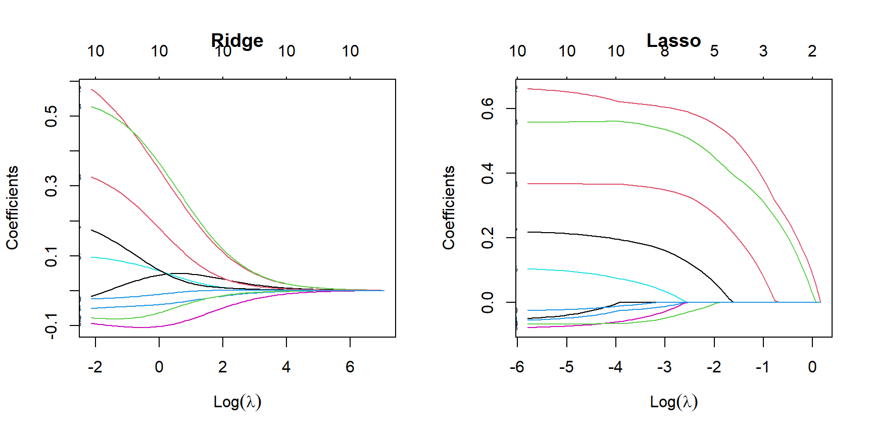
par(mfrow = c(1, 1))Question: Read the lasso panel from right to left (from a big penalty to none). Which covariates enter first?
# choose lambda by 10-fold cross-validation: predict each held-out tenth
set.seed(746)
cv_lasso <- cv.glmnet(X, creepers, family = "poisson", alpha = 1)
plot(cv_lasso)   # left dashed line: lambda.min; right: lambda.1se (simplest within 1 SE)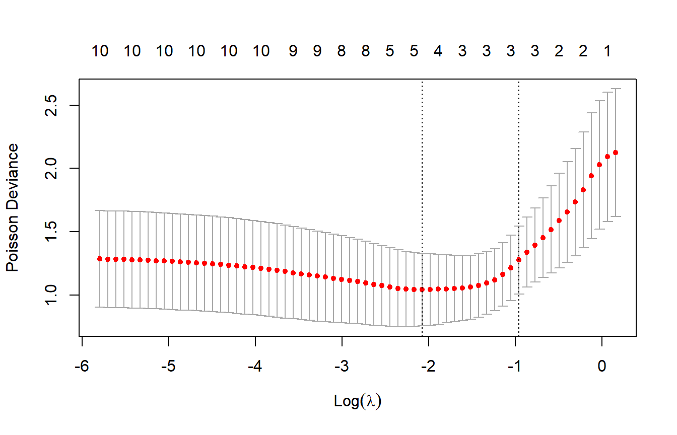
coef_lasso <- coef(cv_lasso, s = "lambda.1se")[-1]

# same cross-validation for ridge (alpha = 0); same folds, so the two are comparable
set.seed(746)
cv_ridge <- cv.glmnet(X, creepers, family = "poisson", alpha = 0)
coef_ridge <- coef(cv_ridge, s = "lambda.1se")[-1]   # try s = "lambda.min": much less shrinkage

round(data.frame(truth = beta_true,
                 MLE = coef(fit_glm)[-1],
                 AIC_best = ifelse(unlist(subsets[which.min(subset_aic), ]), 1, 0),
                 ridge = coef_ridge,
                 lasso = coef_lasso,
                 row.names = covars), 2)
## truth MLE AIC_best ridge lasso
## canopy 0.0 -0.06 0 0.05 0.00
## big_trees 0.5 0.67 1 0.20 0.37
## snags 0.4 0.56 1 0.22 0.30
## shrub 0.0 -0.06 0 -0.03 0.00
## elev 0.0 0.11 0 0.03 0.00
## slope 0.0 -0.08 0 -0.08 0.00
## north 0.0 0.22 1 0.02 0.00
## road_dist 0.3 0.37 1 0.08 0.07
## stream_dist 0.0 -0.07 0 -0.03 0.00
## grazing 0.0 -0.03 0 0.00 0.00Question: The lasso kept road distance but estimates its effect at 0.07; the truth is 0.3. Is the lasso broken?
Neither AIC nor the lasso reliably recovers the true model. In 40 simulated data sets like this one, the AIC-best subset matched the true set of covariates 12 times and the lasso 13 times.
Discussion
Q1. AIC's best creeper model kept northness (several models within 2 units, top weight small); the lasso dropped it. Which covariates would you report as "important," and how would you word it?
Q2. In a real survey, the lasso sets grazing to exactly 0. A manager concludes that expanding grazing won't affect creepers. Do you agree?
Prices, budgets, and cross-validation
These tools come up in a lab on Bd infection in frogs, which fits a logistic model to a 60-pond survey with 8 pond features (data). This part offers another way to picture regularization, as a price or a budget for coefficient size, along with tips for glmnet and an outline of how cross-validation picks the penalty.
Prices and budgets
Think of fitting a model as shopping, with fit as the currency (measured in NLL units). Coefficient size buys a lower NLL: the first bit of a useful coefficient buys a lot, and later bits buy less. A penalty restrains the spending in one of two equivalent ways.
A price. The penalized form, which is what glmnet computes:
\[\min_\beta \; \text{NLL}(\beta) + \lambda \cdot \text{size}(\beta), \qquad \text{size} = \sum_j \beta_j^2 \text{ (ridge) or } \sum_j |\beta_j| \text{ (lasso)}\]
- \(\lambda\) is the price of coefficient size, paid in NLL units.
- There is no spending limit. The fit keeps adding size as long as the next unit lowers the NLL by more than it costs, and stops where the two balance.
- How much gets spent depends on the data: if the fit improves steeply, it pays for a lot of size even at a high price.
- At \(\lambda = 0\), size is free and we get the MLE.
A budget. The constrained form:
\[\min_\beta \; \text{NLL}(\beta) \quad \text{subject to} \quad \sum_j \beta_j^2 \le t^2 \text{ (ridge) or } \sum_j |\beta_j| \le t \text{ (lasso)}\]
- \(t\) is a fixed allowance of coefficient size, with no price. The fit spends it wherever it lowers the NLL most.
- If the MLE fits within the allowance, the limit doesn't bind and we get the MLE. Any \(t\) at least as large as the MLE's size acts like an unlimited budget.
The bridge. Every price has a matching budget that gives the same coefficients.
- Fix \(\lambda\), fit, and add up the size of what was bought. That total is the matching \(t\). (If some point within that budget had a lower NLL, its penalized total would be lower too, so the penalized fit couldn't have been the best.)
- Going the other way, the price that matches a budget \(t\) is how much NLL one more unit of budget would buy.
- As \(\lambda\) rises from 0, the matching \(t\) shrinks from the size of the MLE toward 0. In practice we tune \(\lambda\) (usually by cross-validation); \(t\) pictures how much the fit ended up spending.
Two price schedules.
- Lasso: a flat price. Each unit of \(|\beta_j|\) costs \(\lambda\), starting with the first.
- Ridge: a rising price. Size costs \(\lambda\beta_j^2\), so the next unit costs \(2\lambda\beta_j\): almost nothing near 0, more the more you've already bought.
One coefficient. Take \(\text{NLL}(\beta) = (\beta - 0.4)^2\), so the MLE is 0.4. Raising \(\beta\) from \(b\) lowers the NLL at a rate of \(2(0.4 - b)\) per unit: 0.8 at \(b = 0\), falling to 0 at the MLE.
- Lasso: buy until the rate equals the price, \(2(0.4 - b) = \lambda\), so \(\hat\beta = 0.4 - \lambda/2\) (for \(\lambda < 0.8\)). At \(\lambda = 0.4\), \(\hat\beta = 0.2\).
- Ridge: buy until the rate equals the next unit's price, \(2(0.4 - b) = 2\lambda b\), so \(\hat\beta = 0.4/(1 + \lambda)\). At \(\lambda = 1\), \(\hat\beta = 0.2\).
- Both match a budget of \(t = 0.2\): given an allowance of 0.2 and no price, either penalty would buy the same \(\hat\beta\).
Drag the slider. The left panel shows the lasso objective, with a dot at its minimum; the right panel tracks the lasso and ridge estimates as \(\lambda\) increases.
Question: Why does the lasso buy nothing at all once \(\lambda \ge 0.8\), while ridge always buys some?
Tools for the lab
glmnet(X, y, family = "binomial", alpha = ):alpha = 0is ridge,alpha = 1(the default) is lasso.- For binomial counts,
y = cbind(failures, successes), the reverse ofglm()'s order. glmnetscales the NLL by the sample size, so its \(\lambda\) isn't the \(\lambda\) in a penalty you code by hand. Compare coefficients, not \(\lambda\) values.
Cross-validation
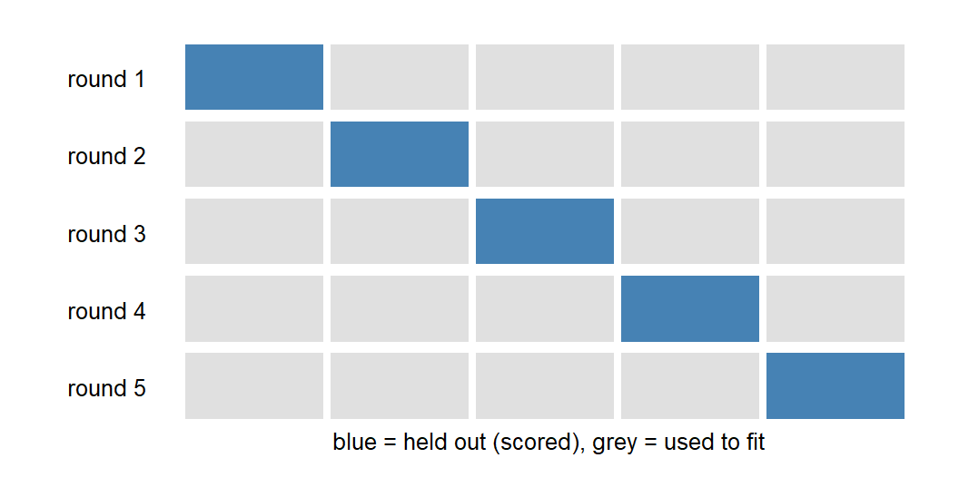
- Fit to 4/5 of the data, score the held-out 1/5 by its NLL, and rotate through all five folds.
- Choose the \(\lambda\) with the best total held-out score.
lambda.1seis the largest \(\lambda\) (the simplest model) whose score is within one SE of the best. - Each held-out fold plays the role of the new plot in the WOD.
- Folds are random, so set a seed to reproduce them.
Bonus: elastic net
The elastic net charges both prices at once, mixed by a second tuning parameter \(\alpha\) between 0 and 1:
\[\min_\beta \; \text{NLL}(\beta) + \lambda \sum_j \Big[\alpha|\beta_j| + (1 - \alpha)\beta_j^2\Big]\]
- \(\lambda\) sets the overall price; \(\alpha\) sets the mix. \(\alpha = 1\) is the lasso and \(\alpha = 0\) is ridge.
- The next unit of \(|\beta_j|\) costs \(\lambda\alpha + 2\lambda(1 - \alpha)|\beta_j|\): a flat fee from the lasso part, plus a rising price from the ridge part.
- The flat fee means a coefficient can still be exactly 0. The rising part keeps any one coefficient from getting large, so the fit spreads its spending more evenly than the lasso does.
For the one-coefficient example, buying until the NLL's rate equals the price gives
\[\hat\beta = \frac{\max(0,\; 0.4 - \lambda\alpha/2)}{1 + \lambda(1 - \alpha)}.\]
The numerator is the lasso's threshold, now reached at \(\lambda = 0.8/\alpha\); the denominator is ridge's proportional shrinkage, applied on top.
In the left panel, the purple line is the price of the next unit and the grey line is what it buys; the estimate sits where they cross, or at 0 if the first unit already costs more than it's worth. Try \(\alpha = 1\) and \(\alpha = 0\) to recover the slider above, then values in between.
In glmnet, the alpha argument is this mix. Its ridge term is written \(\frac{1 - \alpha}{2}\beta_j^2\), half of the one here, so its \(\lambda\) values won't match a hand calculation. cv.glmnet() tunes \(\lambda\) only. To choose \(\alpha\), run it at a few values of alpha with the same foldid and compare the cross-validation scores. The elastic net is a common default when there are many predictors, especially correlated ones, where the lasso and ridge behave differently; the Bd lab works through how.
Causal diagrams: which variables belong in the model?
AIC, cross-validation, and the lasso choose variables by how well they predict. When the question is what would happen if we changed something (protect big trees, close a road), the best predictive model can give the wrong answer. A causal diagram states which variables affect which, and it tells us which variables to include before any model comparison starts.
1. Prediction vs. intervention
A manager might ask where creepers are common (prediction) or what would happen to creepers if we protected big trees (a causal effect). For prediction, any variable that carries information about creeper counts is useful. A regression slope estimates a causal effect only if the model includes the right other variables, and the data alone can't tell us which those are.
A directed acyclic graph (DAG) draws each variable as a node and each direct causal effect as an arrow; "acyclic" means no chain of arrows leads back to where it started. A DAG belongs in the THEORIES box of the workflow: it is a claim about how the system works, made before fitting, and rival theories can have rival DAGs.
2. Three ways a third variable connects
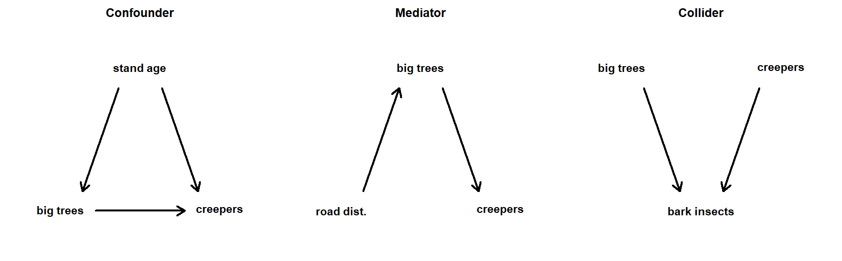
Each panel asks about the effect of big trees (or, in the middle, road access) on creepers.
- Confounder: old stands have big trees, and also other features creepers like. Leave stand age out and big trees get credit for its effect. Include it.
- Mediator: logging near roads removes big trees. To estimate the total effect of road access, leave big trees out; including them blocks the path we want to measure.
- Collider: big trees support more bark insects, and creepers eat them, so insect density depends on both. Leave it out; including it creates an association between big trees and creepers even if there is none.
In short: adjust for common causes of the predictor and the response, and not for consequences of either.
3. A collider fools AIC
Simulated stations where big trees have no effect on creepers, but both affect bark insects:
set.seed(1)
n_sta <- 60
stations <- data.frame(big_trees = rnorm(n_sta))           # standardized
stations$creepers <- rpois(n_sta, exp(1))                   # no effect of big trees
stations$insects <- with(stations,
  0.8 * big_trees - 0.6 * as.vector(scale(creepers)) + rnorm(n_sta, sd = 0.5))

m_trees <- glm(creepers ~ big_trees, family = poisson, data = stations)
m_collider <- glm(creepers ~ big_trees + insects, family = poisson, data = stations)| Big-tree slope | SE | p | AIC |
|---|---|---|---|
| 0.01 | 0.09 | 0.944 | 220.4 |
| 0.38 | 0.11 | 0.001 | 192.4 |
Adding insects lowers AIC by 27.9 units, and the big-tree slope moves from 0.01 to 0.38. AIC is doing its job: insect density does help predict creepers, since creepers deplete insects. But the slope in the better-predicting model is the wrong answer to "what happens if we protect big trees?" The DAG decides which models are eligible to answer a causal question; AIC, cross-validation, or the lasso can then choose among those.
Question: Among stations with the same insect density, why would those with more big trees tend to have more creepers?
Discussion
Q1. A colleague fits creeper counts against all 10 habitat covariates, keeps the model with the lowest AIC, and reports each slope as "the effect of" that covariate on creepers. When is that a fair description, and what would you need to know to check?
Q2. Fire creates snags, and snags help creepers; fire also opens the canopy, which may hurt them. A manager asks whether prescribed burns help creepers. Would you include snag density, canopy cover, both, or neither? Does your answer change if the question is instead whether leaving snags standing after a burn helps?
Bonus: Bayesian model comparison and shrinkage priors
This bonus part brings the same ideas to models fit by MCMC. A ridge penalty is equivalent to a Normal prior, so regularization has a direct Bayesian counterpart. WAIC and LOO estimate predictive performance from the posterior, and shrinkage priors do the job of ridge and the lasso while keeping the full posterior uncertainty.
1. Why not AIC?
AIC needs a single best-fit \(\hat\theta\) and a count of parameters. An MCMC fit gives a whole posterior instead, and priors constrain parameters to different degrees, so the parameter count is no longer clear-cut. WAIC and LOO (section 3) handle both problems.
2. Ridge is a prior
Eight survey routes each report a change in log abundance, \(y_i \sim \text{Normal}(\mu, \sigma = 0.15)\), where \(\mu\) is the regional trend.
- The ridge fit from Regularization, with one parameter: \[\text{PNLL}(\mu) = \sum_{i=1}^n \frac{(y_i - \mu)^2}{2\sigma^2} + \lambda \mu^2\] (the NLL is the Normal density's exponent; the \(\log\sqrt{2\pi\sigma^2}\) terms don't involve \(\mu\), so they drop out).
- Bayes' rule, then \(-\log\): \[P(\mu \mid y) \propto \mathcal{L}(\mu)\, P(\mu) \quad\Rightarrow\quad -\log P(\mu \mid y) = -\log \mathcal{L}(\mu) - \log P(\mu) + \text{const.}\]
- A skeptical prior centered on "no trend," \(\mu \sim \text{Normal}(0, \tau)\): \[-\log P(\mu) = \frac{\mu^2}{2\tau^2} + \text{const.}\]
- Together: \[-\log P(\mu \mid y) = \sum_{i=1}^n \frac{(y_i - \mu)^2}{2\sigma^2} + \frac{\mu^2}{2\tau^2} + \text{const.}\]
- This matches the ridge PNLL when \(\lambda = 1/(2\tau^2)\), so both have the same minimum: the ridge estimate is the posterior mode. A narrow prior means a big penalty; a vague prior (\(\tau \to \infty\)) gives \(\lambda \to 0\), the MLE.
- Setting the derivative to 0: \[\hat\mu = \bar y \cdot \frac{n}{n + \sigma^2/\tau^2}\] This is the MLE times a shrinkage factor below 1. The prior acts like \(\sigma^2/\tau^2\) extra routes that each reported exactly 0.
# 8 survey routes: change in log abundance ~ Normal(mu, sigma = 0.15); mu = regional trend
route_y <- c(0.12, -0.05, 0.20, 0.08, -0.10, 0.15, 0.02, 0.10)
sigma <- 0.15
tau <- 0.05                       # prior: mu ~ Normal(0, tau)
lambda <- 1 / (2 * tau^2)         # ridge penalty that matches it
nll_mu <- function(mu) sapply(mu, function(m) sum((route_y - m)^2) / (2 * sigma^2))
pnll_mu <- function(mu) nll_mu(mu) + lambda * mu^2                       # ridge
neg_log_post <- function(mu) nll_mu(mu) - dnorm(mu, 0, tau, log = TRUE)  # Bayes
c(MLE = mean(route_y),
  ridge = optimize(pnll_mu, c(-1, 1))$minimum,
  posterior_mode = optimize(neg_log_post, c(-1, 1))$minimum)
## MLE ridge posterior_mode
## 0.06500000 0.03058824 0.03058824Drag the prior SD \(\tau\). The posterior, and the ridge \(\lambda\) that matches it, shift between the data and 0.
Question: Which prior matches the lasso penalty, \(\lambda|\mu|\)?
3. WAIC and LOO
- Score: the expected log predictive density (elpd). For each data point, average its likelihood over the posterior draws, take the log, and sum over points. Higher is better; the "IC" versions are \(-2 \times\) elpd.
- Penalty: effective number of parameters, estimated from the posterior.
- DIC (Bolker 6.6.3): \(p_D\) = mean deviance minus the deviance at the posterior means.
- WAIC: \(p_{\text{waic}}\) = the summed posterior variance of each point's log likelihood.
- LOO: approximates refitting the model without each point (PSIS). Pareto \(k > 0.7\) flags points where the approximation fails.
- Stan has to save
log_lik[i]for every observation, ingenerated quantities.
library(cmdstanr)
library(loo)

# fir NegBin power law; G = 1: one a, b, k for all trees; G = 2: separate for wave/non-wave
fir_code <- "
data {
  int<lower=1> N;
  int<lower=1> G;
  array[N] int<lower=0> cones;
  vector<lower=0>[N] dbh;
  array[N] int<lower=1, upper=G> grp;
}
parameters {
  vector[G] log_a;
  vector[G] b;
  vector<lower=0>[G] k;
}
model {
  log_a ~ normal(0, 5);
  b ~ normal(0, 5);
  k ~ exponential(0.1);
  cones ~ neg_binomial_2(exp(log_a[grp]) .* pow(dbh, b[grp]), k[grp]);
}
generated quantities {
  vector[N] log_lik;    // one value per tree, for WAIC and LOO
  for (i in 1:N)
    log_lik[i] = neg_binomial_2_lpmf(cones[i] | exp(log_a[grp[i]]) * dbh[i]^b[grp[i]], k[grp[i]]);
}
"
fir_model <- cmdstan_model(write_stan_file(fir_code))
fit_fir <- function(G) {
  grp <- if (G == 1) rep(1L, nrow(fir)) else wave
  fir_model$sample(data = list(N = nrow(fir), G = G, cones = fir$TOTCONES, dbh = fir$DBH,
                               grp = grp),
                   chains = 4, parallel_chains = 4, seed = 746, refresh = 0,
                   show_messages = FALSE)
}
fit_nowave_b <- fit_fir(1)
fit_full_b <- fit_fir(2)
# DIC (Bolker 6.6.3): pD = mean deviance - deviance at posterior means; DIC = Dhat + 2 pD
dic <- function(fit, G) {
grp <- if (G == 1) rep(1L, nrow(fir)) else wave
d_bar <- mean(-2 * rowSums(fit$draws("log_lik", format = "matrix")))
pm <- function(v) colMeans(fit$draws(v, format = "matrix"))
d_hat <- -2 * sum(dnbinom(fir$TOTCONES, mu = exp(pm("log_a")[grp]) * fir$DBH^pm("b")[grp],
size = pm("k")[grp], log = TRUE))
c(DIC = d_hat + 2 * (d_bar - d_hat), pD = d_bar - d_hat)
}
waic_nowave <- waic(fit_nowave_b$draws("log_lik", format = "matrix"))
waic_full <- waic(fit_full_b$draws("log_lik", format = "matrix"))
loo_nowave <- fit_nowave_b$loo()
loo_full <- fit_full_b$loo()
loo_nowave # elpd_loo, p_loo, looic, and the Pareto k check##
## Computed from 4000 by 242 log-likelihood matrix.
##
## Estimate SE
## elpd_loo -1139.3 15.1
## p_loo 3.5 0.6
## looic 2278.6 30.1
## ------
## MCSE of elpd_loo is 0.0.
## MCSE and ESS estimates assume MCMC draws (r_eff in [0.3, 1.1]).
##
## All Pareto k estimates are good (k < 0.7).
## See help('pareto-k-diagnostic') for details.# the same two models, four ways (lower is better; penalties: k, pD, p_waic, p_loo)
ic_tab <- rbind(
AIC = aic_tab$AIC[match(c("no_wave", "full"), aic_tab$model)],
DIC = c(dic(fit_nowave_b, 1)["DIC"], dic(fit_full_b, 2)["DIC"]),
WAIC = c(waic_nowave$estimates["waic", 1], waic_full$estimates["waic", 1]),
LOOIC = c(loo_nowave$estimates["looic", 1], loo_full$estimates["looic", 1]))
colnames(ic_tab) <- c("no_wave", "full")
round(ic_tab, 1)## no_wave full
## AIC 2278.0 2282.0
## DIC 2278.0 2281.9
## WAIC 2278.6 2282.7
## LOOIC 2278.6 2282.7fir_comp <- loo_compare(list(no_wave = loo_nowave, full = loo_full))
fir_comp## elpd_diff se_diff
## no_wave 0.0 0.0
## full -2.1 1.8Question: The full model is 2.1 elpd behind, SE 1.8. What can you conclude?
Unlike AIC, LOO gives a standard error for the difference between two models.
4. Shrinkage priors
The prior's scale plays the role of \(\lambda\): a Normal prior on the slopes corresponds to ridge, a Laplace prior to the lasso. Here are the brown creepers from Regularization again, with three different priors on the 10 slopes:
# creepers again: Poisson regression; prior on the slopes is Normal(0, s) or Laplace(0, s)
pois_code <- "
data {
  int<lower=1> N;
  int<lower=1> K;
  matrix[N, K] X;
  array[N] int<lower=0> y;
  int<lower=1, upper=2> prior;    // 1 = Normal, 2 = Laplace
  real<lower=0> s;
}
parameters {
  real b0;
  vector[K] beta;
}
model {
  b0 ~ normal(0, 5);
  if (prior == 1) beta ~ normal(0, s);
  else beta ~ double_exponential(0, s);
  y ~ poisson_log(b0 + X * beta);
}
generated quantities {
  vector[N] log_lik;
  for (i in 1:N) log_lik[i] = poisson_log_lpmf(y[i] | b0 + X[i] * beta);
}
"
pois_model <- cmdstan_model(write_stan_file(pois_code))
fit_creepers <- function(prior, s) {
  pois_model$sample(data = list(N = 50, K = 10, X = X, y = creepers, prior = prior, s = s),
                    chains = 4, parallel_chains = 4, seed = 746, refresh = 0,
                    show_messages = FALSE)
}
fits_shrink <- list(vague = fit_creepers(1, 10), normal = fit_creepers(1, 0.2),
                    laplace = fit_creepers(2, 0.15))
# posterior medians and 90% intervals for each slope, under each prior; x = truth
post_sum <- lapply(fits_shrink, function(f) {
as.matrix(f$summary("beta", "median", ~quantile(.x, c(0.05, 0.95)))[, -1])
})
par(mar = c(4, 7, 1, 1))
plot(NA, xlim = c(-0.5, 1), ylim = c(0.5, 10.5), yaxt = "n", xlab = "Slope (per SD)", ylab = "")
axis(2, at = 10:1, labels = covars, las = 1, cex.axis = 0.8)
abline(v = 0, col = "grey70")
offsets <- c(vague = 0.25, normal = 0, laplace = -0.25)
for (p in names(post_sum)) {
yy <- (10:1) + offsets[p]
segments(post_sum[[p]][, 2], yy, post_sum[[p]][, 3], yy, lwd = 2, col = match(p, names(post_sum)))
points(post_sum[[p]][, 1], yy, pch = 19, col = match(p, names(post_sum)))
}
points(beta_true, 10:1, pch = 4, cex = 1.3, lwd = 2)
points(coef_lasso, 10:1, pch = 2)
legend("bottomright", c("vague prior", "Normal(0, 0.2)", "Laplace(0, 0.15)", "truth", "glmnet lasso"),
col = c(1:3, 1, 1), pch = c(19, 19, 19, 4, 2), bty = "n", cex = 0.8)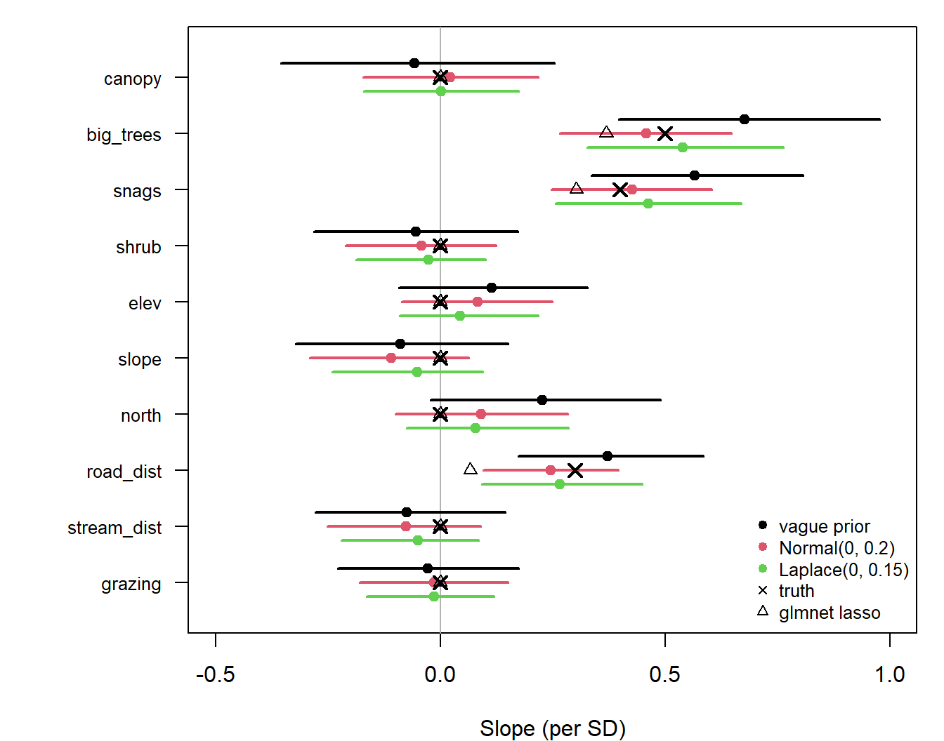
sapply(fits_shrink, function(f) f$loo()$estimates["p_loo", 1]) # effective parameters shrink## vague normal laplace
## 9.141144 7.834112 7.121993loo_compare(lapply(fits_shrink, function(f) f$loo()))## elpd_diff se_diff
## laplace 0.0 0.0
## normal -1.5 1.2
## vague -1.5 1.6Question: The cross-validated lasso in Regularization set northness to exactly 0. The Laplace posterior says 0.08 (90% interval -0.07 to 0.28). Which is more honest?
Horseshoe prior (sketch only): a taller spike at 0 plus heavier tails, so small effects shrink hard and large ones barely shrink.
# prior shapes: Normal, Laplace, horseshoe (simulated: Normal with half-Cauchy scale)
set.seed(746)
hs <- rnorm(1e6, 0, 0.1 * abs(rcauchy(1e6)))
curve(dnorm(x, 0, 0.2), -1, 1, n = 501, lwd = 2, ylim = c(0, 6), xlab = "Slope", ylab = "Prior density")
curve(dexp(abs(x), 1 / 0.15) / 2, -1, 1, n = 501, add = TRUE, lwd = 2, col = 3)
lines(density(hs[abs(hs) < 1], bw = 0.01, n = 1024), lwd = 2, col = 4)
legend("topright", c("Normal (ridge)", "Laplace (lasso)", "horseshoe"), col = c(1, 3, 4),
       lwd = 2, bty = "n")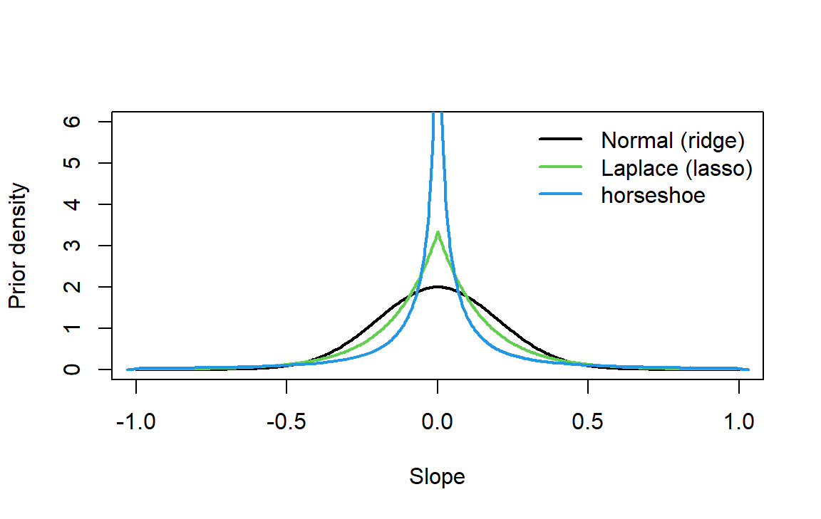
Choosing the prior scale amounts to choosing \(\lambda\). Scales can be compared by LOO, or the scale can be estimated from the data with a hierarchical prior (covered later in the course).
Discussion
Q1. LOO prefers the no-wave fir model by 2.1 elpd (SE 1.8). A colleague writes "wave regeneration has no effect on cone production." Do you agree?
Q2. With a Laplace prior, northness gets a posterior median of 0.08; the cross-validated lasso said exactly 0. Which would you report, and why?
Bayes factors and RJMCMC
- A Bayes factor is a ratio of marginal likelihoods (the likelihood averaged over the prior). It is sensitive to vague priors and hard to compute (Bolker 6.6.3).
- RJMCMC and spike-and-slab priors let the sampler jump between models, giving posterior model probabilities. They need discrete parameters, so they run in JAGS or NIMBLE rather than Stan.