Download the code here: rfregression.R

Download the data here: ET_data.csv

Random Forest regression is done as follows

split the data set into train and test.
create Random Forest object
plot oob error rate
tune Random Forests finding optimal mtry.
do cross validation on complete dataset.
plot variable importance.

library(randomForest)

## randomForest 4.7-1.1

## Type rfNews() to see new features/changes/bug fixes.

library(rfUtilities)

## Warning: package 'rfUtilities' was built under R version 4.3.2

my_data = read.csv("ET_data.csv")
my_data = na.omit(my_data)
# Initialize empty training and test sets
train_set <- data.frame()
test_set <- data.frame()

# Specify the number of rows to include in each set alternately
rows_per_set <- 3

# Create alternating sets
for (i in seq(1, nrow(my_data), by = rows_per_set * 2)) {
  test_indices <- i:(i + rows_per_set - 1)
  train_indices <- (i + rows_per_set):(i + rows_per_set * 2 - 1)

  test_set <- rbind(test_set, my_data[test_indices, , drop = FALSE])
  train_set <- rbind(train_set, my_data[train_indices, , drop = FALSE])
}

train_set <- na.omit(train_set)
set.seed(123)
rf <- randomForest(data = train_set ,x = train_set[,c(1,3:8)],y = train_set$ET,ntree = 600,mtry = 2,importance = TRUE,proximity = TRUE)
print(rf)

## 
## Call:
##  randomForest(x = train_set[, c(1, 3:8)], y = train_set$ET, ntree = 600,      mtry = 2, importance = TRUE, proximity = TRUE, data = train_set) 
##                Type of random forest: regression
##                      Number of trees: 600
## No. of variables tried at each split: 2
## 
##           Mean of squared residuals: 1.849529
##                     % Var explained: 78.8

Plotting OOB error rate

plot(rf)

Tuning RF

set.seed(123)
tuneRF(y = train_set$ET,x = train_set[,c(1,3:8)],mtryStart = 2,stepFactor = 3,trace = TRUE,plot = TRUE, ntreeTry = 600 )

## mtry = 2  OOB error = 1.835301 
## Searching left ...
## mtry = 1     OOB error = 1.940607 
## -0.0573783 0.05 
## Searching right ...
## mtry = 6     OOB error = 1.934177 
## -0.05387467 0.05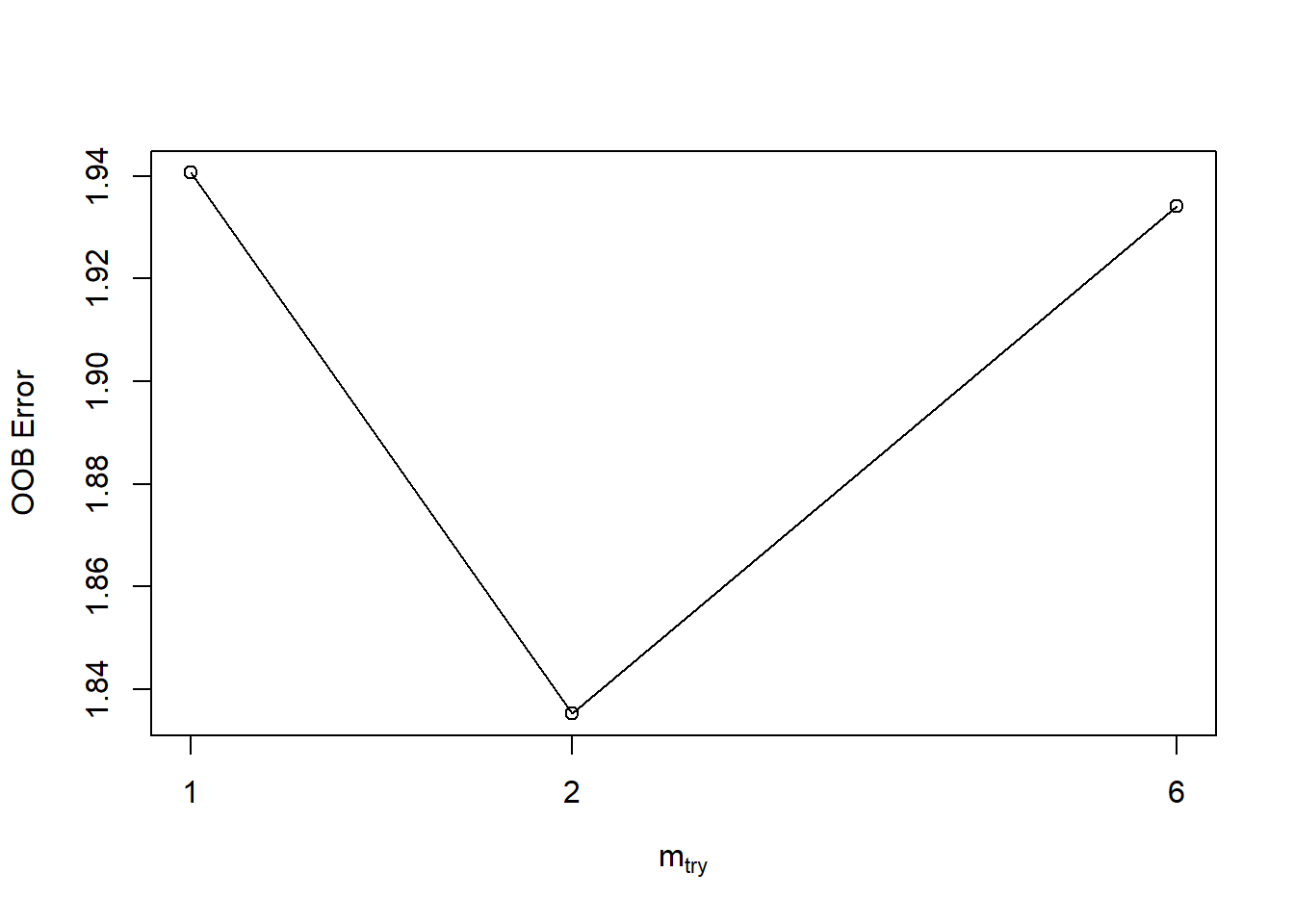

##   mtry OOBError
## 1    1 1.940607
## 2    2 1.835301
## 6    6 1.934177

Cross validation

We trained the model with only train dataset.
we are using the complete data set to do cross validation.

cv <- rf.crossValidation(x= rf, xdata = my_data[,c(1,3:8)],ydata = my_data$ET,p = 0.2, n = 99, seed = 123)

## running: regression cross-validation with 99 iterations

fit.var.exp: Percent variance explained from the specified fit model. This metric typically represents the proportion of variance in the dependent variable that is explained by the model.

$\text{Percent Variance Explained} = 100 \times \left(1 -\frac{\\text{Residual Sum of Squares}}{\text{Total Sum of Squares}}\right)$

mean(cv$fit.var.exp)

## [1] 78.8

fit.mse: Mean Squared Error from the specified fit model. MSE is a measure of the average squared differences between observed and predicted values. It is commonly used as a measure of the model's accuracy.

$\text{Mean Squared Error (MSE)} = \frac{1}{n} \sum_{i=1}^{n} (y_i - \hat{y}_i)^2 $

mean(cv$fit.mse)

## [1] 1.862548

y.rmse: Root Mean Squared Error (observed vs. predicted) from each Bootstrap iteration (cross-validation). RMSE is similar to MSE but provides a measure in the original units of the response variable.

$\text{Root Mean Squared Error (RMSE)} = \sqrt{\frac{1}{n} \sum_{i=1}^{n} (y_i - \hat{y}_i)^2}$

mean(cv$y.rmse)

## [1] 1.273641

y.mbe: Mean Bias Error from each Bootstrapped model. Bias is the difference between the average prediction and the true value.

$\text{Mean Bias Error (MBE)} = \frac{1}{n} \sum_{i=1}^{n} (y_i - \hat{y}_i)$

mean(cv$y.mbe)

## [1] 0.01062168

y.mae: Mean Absolute Error from each Bootstrapped model. MAE is the average of the absolute differences between observed and predicted values. It is less sensitive to outliers than MSE.

$\text{Mean Absolute Error (MAE)} = \frac{1}{n} \sum_{i=1}^{n} |y_i - \hat{y}_i|$

mean(cv$y.mae)

## [1] 0.8425645

The Kolmogorov-Smirnov (KS) test statistic ($D$) is a measure of the maximum absolute difference between the cumulative distribution functions (CDFs) of two datasets. The KS test is often used to assess whether a sample comes from a particular distribution or to compare two samples. Here's how to interpret the (D) statistic:
Larger ($D$): A larger ($D$) value indicates a greater discrepancy between the two empirical cumulative distribution functions. This suggests that the two samples are less likely to come from the same underlying distribution.
Smaller ($D$): A smaller ($D$) value indicates a smaller discrepancy between the two CDFs, suggesting that the samples are more similar in terms of their distribution.

mean(cv$D)

## [1] 0.1249158

p.val: The p-value represents the probability of observing a ($D$) value as extreme as the one computed, assuming that the two samples are drawn from the same distribution.
- Small p-value: Indicates evidence to reject the null hypothesis that the two samples come from the same distribution.
- Large p-value: Suggests that there is insufficient evidence to reject the null hypothesis.

Null Hypothesis: The null hypothesis of the KS test is that the two samples come from the same distribution.

mean(cv$p.val)

## [1] 0.3423244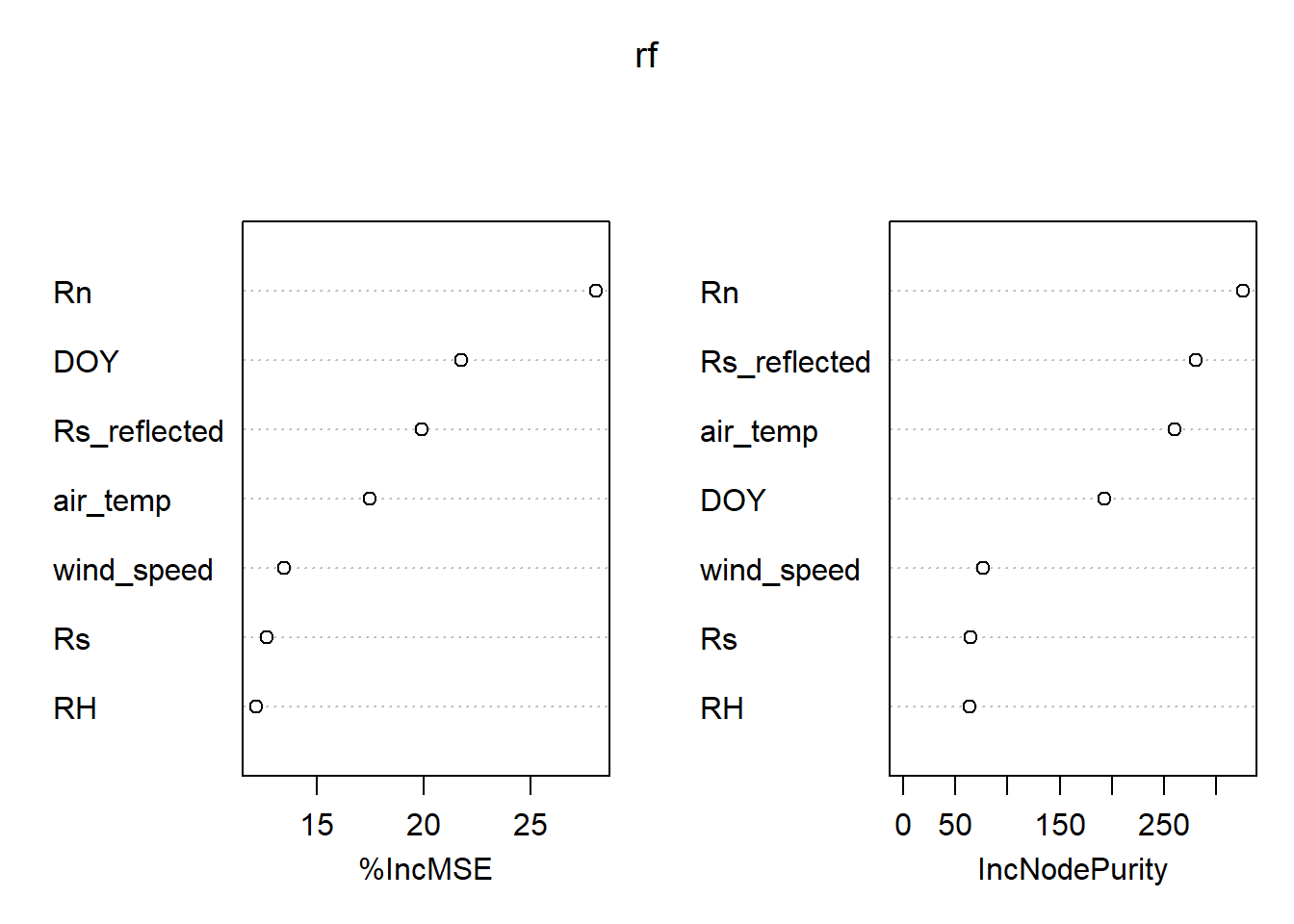

Variable Importance Plot

varImpPlot(rf)

Exercise

# Start of exercise ------------------------

library(randomForest)
library(rfUtilities)

my_data = read.csv("ET_data.csv")   # replace with your specific filepath if needed
my_data = na.omit(my_data)
# Initialize empty training and test sets
train_set <- data.frame()
test_set <- data.frame()

# Specify the number of rows to include in each set alternately
rows_per_set <- 3

# Create alternating sets
for (i in seq(1, nrow(my_data), by = rows_per_set * 2)) {
  test_indices <- i:(i + rows_per_set - 1)
  train_indices <- (i + rows_per_set):(i + rows_per_set * 2 - 1)

  test_set <- rbind(test_set, my_data[test_indices, , drop = FALSE])
  train_set <- rbind(train_set, my_data[train_indices, , drop = FALSE])
}

train_set <- na.omit(train_set)
set.seed(123)
rf <- randomForest(data = train_set ,x = train_set[,c(1,3:8)],y = train_set$ET,ntree = 600,mtry = 2,importance = TRUE,proximity = TRUE)
print(rf)

## 
## Call:
##  randomForest(x = train_set[, c(1, 3:8)], y = train_set$ET, ntree = 600,      mtry = 2, importance = TRUE, proximity = TRUE, data = train_set) 
##                Type of random forest: regression
##                      Number of trees: 600
## No. of variables tried at each split: 2
## 
##           Mean of squared residuals: 1.849529
##                     % Var explained: 78.8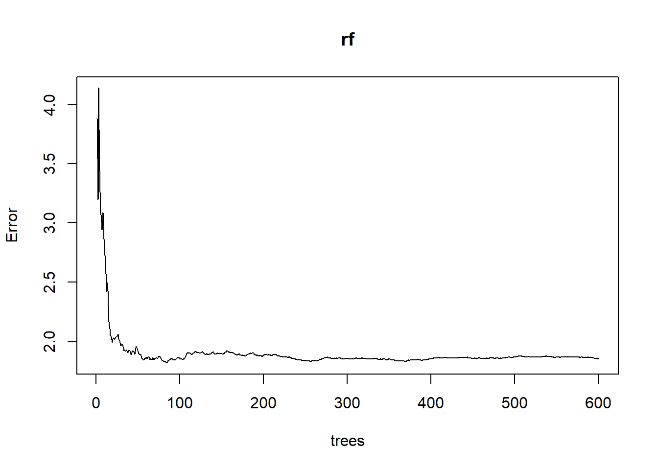

# Plotting OOB error rate

plot(rf)

# Tuning RF

set.seed(123)
tuneRF(y = train_set$ET,x = train_set[,c(1,3:8)],,mtryStart = 2,stepFactor = 3,trace = TRUE,plot = TRUE, ntreeTry = 600 )

## mtry = 2  OOB error = 1.835301 
## Searching left ...
## mtry = 1     OOB error = 1.940607 
## -0.0573783 0.05 
## Searching right ...
## mtry = 6     OOB error = 1.934177 
## -0.05387467 0.05

##   mtry OOBError
## 1    1 1.940607
## 2    2 1.835301
## 6    6 1.934177

# Cross validation

#- We trained the model with only train dataset.
#- we are using the complete data set to do cross validation.


cv <- rf.crossValidation(x= rf, xdata = train_set[,c(1,3:8)],ydata = train_set$ET,p = 0.2, n = 99, seed = 123)

## running: regression cross-validation with 99 iterations

#fit.var.exp
mean(cv$fit.var.exp)

## [1] 78.8

#fit.mse
mean(cv$fit.mse)

## [1] 1.862548

#y.rmse
mean(cv$y.rmse)

## [1] 1.375269

#y.mbe
mean(cv$y.mbe)

## [1] 0.02598397

#y.mae
mean(cv$y.mae)

## [1] 0.9622028

# D (Kolmogorov-Smirnov distribution test)
mean(cv$D)

## [1] 0.1744108

#p.val(p-value for the Kolmogorov-Smirnov distribution test)
mean(cv$p.val)

## [1] 0.3528096

#Variable Importance Plot
varImpPlot(rf)

Random Forest Regression

Elena cox, Katarena Matos Meira, Mahipal Reddy Ramireddy

Plotting OOB error rate

Tuning RF

Cross validation

Variable Importance Plot

Exercise