Geostatistical Modeling Using R-INLA: Malaria Prevalence in The Gambia
Melissa Schwan
2023-11-28
You can download the code here: SpatialRegression.R
Introduction
In this demo we will do a spatial regression model using R-INLA. You can download R-INLA by copying the commented code below into your console and running it, or by visiting the R-INLA download site: https://www.r-inla.org/download-install
#install.packages("INLA",repos=c(getOption("repos"),INLA="https://inla.r-inla-download.org/R/stable"), dep=TRUE)We will use a geostatistical model to predict malaria prevalence in The Gambia. We will use Integrated Nested Laplace Approximation (INLA), which is a method for approximating model parameters in a Bayesian framework. The method here uses a stochastic partial differential equation (SPDE) approach to estimate continuous spatial effects using discrete points created by a mesh, and basis functions, resulting in a random effects surface which goes into our INLA model. We are using the gambia dataset from the package ‘geoR’ which consists of blood test results from children screened for malaria in 65 towns in The Gambia. In addition, we are using an elevation raster downloaded with the ‘geodata’ package. Following the SPDE approach, we build a triangulated mesh to cover The Gambia. Then we make a projection matrix and stack the data for the model. Then we use the results to obtain predictions, and show 95% Credible Intervals for uncertainty.
This tutorial is modified from chapter 9 of Paula Moraga’s book “Geospatial Health Data: Modeling and Visualization with R-INLA and Shiny”, available here: https://www.paulamoraga.com/book-geospatial/sec-geostatisticaldataexamplespatial.html
You will need several packages for this tutorial:
Gambia Data
Load the gambia dataset, from the ‘geoR’ package, and look at it.
##             x       y pos  age netuse treated green phc
## 1850 349631.3 1458055   1 1783      0       0 40.85   1
## 1851 349631.3 1458055   0  404      1       0 40.85   1
## 1852 349631.3 1458055   0  452      1       0 40.85   1
## 1853 349631.3 1458055   1  566      1       0 40.85   1
## 1854 349631.3 1458055   0  598      1       0 40.85   1
## 1855 349631.3 1458055   1  590      1       0 40.85   1
The variables in the gambia dataset:
x: x coordinate of village in UTM (zone 28)
y: y coordinate of village in UTM (zone 28)
pos: presence (1) or absence (0) of malaria in blood
sample. We calculate prevalence from this variable.
age: age of the child, in days
netuse: indicator whether child sleeps under a net (1)
or not (0)
treated: indicator of whether net is treated
green: satellite data, measure of greenness in the
vicinity of the village
phc: indicator of whether a health center is present in
village
Data Preparation
In this dataset, each observation is for an individual blood
test.
We want to do our analysis on malaria prevalence at the village level.
Prevalence is the number of positive tests out of total tests, for each
village.
To do this we will make a new dataframe with data at the village
level.
First take a look at the number of unique locations.
## [1] 65 2There are 65 unique locations. So our dataframe needs to have 65
rows, and 5 columns including:
x and y: 2 columns for x and y
coordinates, in this order
total: total number of tests
positive: number of positive tests
prev: prevalence of malaria, calculated
positive/total
For the lab-part 1
Are there any other variables you would want to include? How can you include them on a per-village scale? I included code to add netuse and greenness to the data frame, what others would you add? You may even want to add that code here so you have it in your data frame.
# For the lab-part 1, different variables, consider other models----
# dplyr and summary statistics to create the new columns
d <- group_by(gambia, x, y) %>%
  summarize(
    total = n(),
    positive = sum(pos),
    prev = positive / total
    #,netuse = mean(netuse) # for the lab, you could include these
    #,greenness = mean(green)
  )
head(d)
## # A tibble: 6 × 5
## # Groups: x [6]
## x y total positive prev
## <dbl> <dbl> <int> <dbl> <dbl>
## 1 349631. 1458055 33 17 0.515
## 2 358543. 1460112 63 19 0.302
## 3 360308. 1460026 17 7 0.412
## 4 363796. 1496919 24 8 0.333
## 5 366400. 1460248 26 10 0.385
## 6 366688. 1463002 18 7 0.389Geometry, Coordinates, and Transforming the Coord. System
With package ‘sf’. We will need to first create geometric points from
our x,y data, then specify the coordinate reference system (UTM Zone 28
North), then transform the points into a long,lat coordinate system
(we’ll use WGS84).
Then we’ll add the long and lat columns to our data frame.
# create geometric points from XY
pts <-
  st_multipoint(x = as.matrix(d[,1:2]), dim="XY")
# create spatially referenced points: these are in UTM Zone 28 N
sp <-
  st_sfc(pts, crs = "+proj=utm +zone=28")
# transform to long lat crs: WGS84
sp_tr <-
  st_transform(sp, crs = "+proj=longlat +datum=WGS84")
# add long, lat columns to data frame
d[, c("long", "lat")] <- st_coordinates(sp_tr)[,1:2]
head(d)
## # A tibble: 6 × 7
## # Groups: x [6]
## x y total positive prev long lat
## <dbl> <dbl> <int> <dbl> <dbl> <dbl> <dbl>
## 1 349631. 1458055 33 17 0.515 -16.4 13.2
## 2 358543. 1460112 63 19 0.302 -16.3 13.2
## 3 360308. 1460026 17 7 0.412 -16.3 13.2
## 4 363796. 1496919 24 8 0.333 -16.3 13.5
## 5 366400. 1460248 26 10 0.385 -16.2 13.2
## 6 366688. 1463002 18 7 0.389 -16.2 13.2Map of Malaria Prevalence with package ‘leaflet’
In this tutorial we’re using the package ‘leaflet’ to map data. It looks tidy and is very nice for including interactive maps into your reports. Also check out ‘leafsync’ for viewing multiple synchronized panes of interactive maps to show multiple aspects of your spatial data.
pal <- colorBin("viridis", bins = c(0, 0.25, 0.5, 0.75, 1))
leaflet(d) %>%
  addProviderTiles(providers$CartoDB.Positron) %>%
  addCircles(lng = ~long, lat = ~lat, color = ~ pal(prev)) %>%
  addLegend("bottomright",
            pal = pal, values = ~prev,
            title = "Malaria Prevalence"
  ) %>%
  addScaleBar(position = c("bottomleft"))
Figure 1: Map of Malaria Prevalence in The Gambia
Fixed Effects: Elevation from package ‘geodata’
In this demo, we model elevation as a fixed effect, so here we get an elevation raster with function geodata::elevation_30s(), and mask it to only include data for The Gambia region using the country code “GMB”. The ‘geodata’ package has functions for downloading different types of geographic data. The ‘terra’ package has functions to aid working with rasters.
r <- elevation_30s(country = "GMB",
                   path = tempdir(), mask = TRUE)

pal <- colorNumeric("viridis", values(r),
                    na.color = "transparent"
)
# map elevation raster
leaflet() %>%
  addProviderTiles(providers$CartoDB.Positron) %>%
  addRasterImage(r, colors = pal, opacity = 0.5) %>%
  addLegend("bottomright",
            pal = pal, values = values(r),
            title = "Altitude (m)"
  ) %>%
  addScaleBar(position = c("bottomleft"))
Figure 2: Elevation in The Gambia. Data source SRTM.
# extract elevation for all observations and add "alt" to dataframe
d["alt"] <-
  terra::extract(r, d[, c("long", "lat")],
                 list=T, ID=F, method="bilinear")
head(d)
## # A tibble: 6 × 8
## # Groups: x [6]
## x y total positive prev long lat alt
## <dbl> <dbl> <int> <dbl> <dbl> <dbl> <dbl> <dbl>
## 1 349631. 1458055 33 17 0.515 -16.4 13.2 15.8
## 2 358543. 1460112 63 19 0.302 -16.3 13.2 32.1
## 3 360308. 1460026 17 7 0.412 -16.3 13.2 32.2
## 4 363796. 1496919 24 8 0.333 -16.3 13.5 19.5
## 5 366400. 1460248 26 10 0.385 -16.2 13.2 26.0
## 6 366688. 1463002 18 7 0.389 -16.2 13.2 18.1For the lab-part 2 “MyRaster”
One option for the lab: Try a different covariate to model as a fixed effect and see how this differs from the first model where we use elevation, or include them both. For geo data, the package ‘geodata’ has more raster datasets available, and you can explore them here: https://rdrr.io/github/rspatial/geodata/man/
I’ve included code here to help. You can use it as is if you want to look at wind, or change it to look at a different variable.
# For the lab-part 2, "MyRaster" ----

# help(package="geodata") # click on a dataset help page to learn about the dataset and choose a variable
#
# ## here's an example:
# gdata <- worldclim_country(country = "GMB",
#                                var="wind", # choose anything!
#                                path = tempdir(),
#                                version=2.1,
#                                mask = TRUE)
# ## wind is average monthly data, so it has 12 layers. You can use terra::subset() to choose one or more months (layers) and average across them for seasonal data
#
# my_raster <- mean(subset(x=gdata, subset=c(7,8,9,10))) #subsetting July-October and taking the mean, so we will have July-October wind speeds
#
# pal <- colorNumeric("viridis", values(my_raster),
#                     na.color = "transparent"
# )
# # map my_raster
# leaflet() %>%
#   addProviderTiles(providers$CartoDB.Positron) %>%
#   addRasterImage(my_raster, colors = pal, opacity = 0.5) %>%
#   addLegend("bottomright",
#             pal = pal, values = values(my_raster),
#             title = "JASO wind (m/s)" # change to the units for your variable
#   ) %>%
#   addScaleBar(position = c("bottomleft"))
# # extract measurement for all observations and add this variable to dataframe
# d["wind"] <- # change this to reflect the variable you chose
#   terra::extract(my_raster, d[, c("long", "lat")],
#                  list=T, ID=F, method="bilinear")
# head(d)
Modeling Malaria Prevalence
Now we can get to the modeling!
Specify Model
The number of positive malaria tests (pos_i) out of the total number sampled (N_i), conditional on the true prevalence at a certain location prev(x_i), follows a binomial distribution, with a logit link.
pos_i|prev(x_i) ~ Binomial(N_i, prev(x_i)) logit(prev(x_i) = beta0 + beta1*altitude + s(x_i)
beta0 = intercept
beta1 = coefficient for altitude
s = spatial random effect
Create the Triangulated Mesh
We build a triangulated mesh whose vertices will
create the discrete points to which the basis functions will be fitted.
This will become a continuous Gaussian random field which represents the
spatial random effect. This approach might sound familiar: nodes and
splines.
We have set max.edge = c(0.1,5) to make smaller triangles inside the
region and larger ones in the extension. This cuts down on computation
in the outer region where there are no observations. You can
play around with the max.edge values and see how it affects your
mesh.
cutoff = 0.01 avoids making many small triangles in areas where there
are lots of observations close together.
### Build the mesh ----
coo <- cbind(d$long, d$lat) # coordinates of observations
mesh <- inla.mesh.2d(loc = coo,
                     # loc is coordinates to start the mesh
                     max.edge = c(0.1, 5),
                     # max.edge-play around with these values and see
                     cutoff = 0.01
)
mesh$n
## [1] 673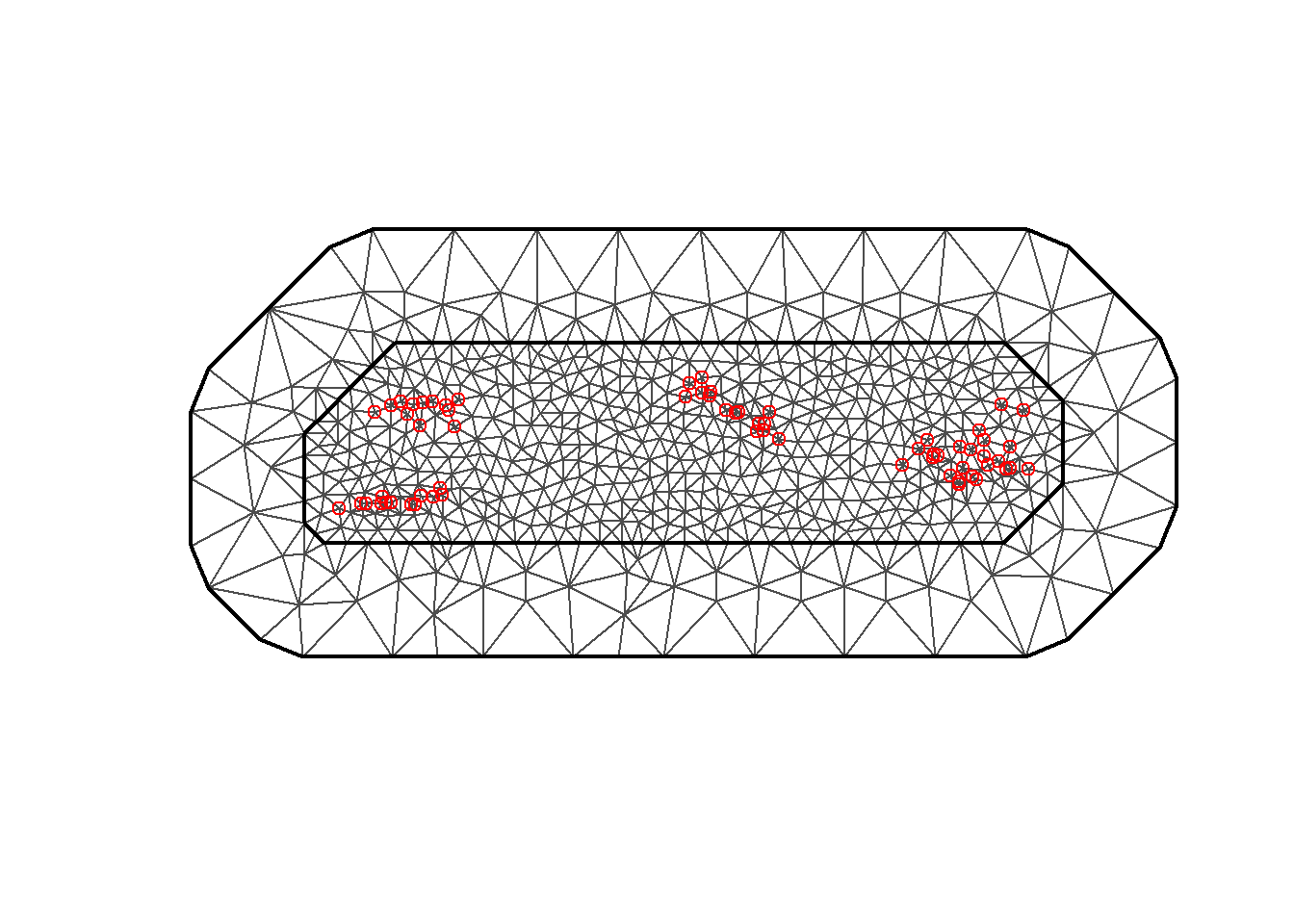
Figure 2: Triangulated Mesh used for the SPDE model.
Build the SPDE model on the mesh
INLA uses a stochastic partial differential equation
(SPDE), some complex math, to model the spatial random effect,
the Gaussian random field.
The spatial effect function is a “zero-mean, Gaussian process with
Matern covariance”.
The alpha parameter is related to the smoothness parameter v for the
random process. And d is the dimension of the random effect.
\[\alpha = v + \frac{d}{2}\] In our
example, v=1, d=2, so alpha = 1+2/2 = 2.
within the inla.spde2.matern() you can set priors for the spatial
effect with the following arguments.
prior.variance.nominal=
prior.range.nominal=
Setting these priors has a large effect on the fitted model. You can try
setting them, and see what effect it has on your model output.
### Build the SPDE model on the mesh ----
# SPDE model: here is the spatial effect!!
spde <-
  inla.spde2.matern(mesh = mesh,
                    alpha = 2, # 0 > alpha ≥ 2
                    #prior.variance.nominal = 1, # nominal prior mean for the field variance, sigma
                    #prior.range.nominal = NULL, # nominal prior mean for the spatial range
                    constr = TRUE) # constr imposes an integrate-to-zero constraint for our model
### Index the SPDE ----
indexs <-
  inla.spde.make.index("s", spde$n.spde)
lengths(indexs)
## s s.group s.repl
## 673 673 673Projection Matrix A
The projection matrix projects the spatially continuous Gaussian random field from the observations to the mesh nodes. It contains the basis functions that will be fitted to the nodes of the mesh.
Prediction Matrix Ap
The prediction matrix has the coordinates of the positions where we will predict the malaria prevalence values.
### Prediction data ----

dp <- terra::as.points(r) # this makes the r raster into a vector of points
dim(dp)
## [1] 12847 1ra <- terra::aggregate(r, fact = 4, fun = mean) # reduce the number of raster cells, factor 4 combines 4x4 cells of raster into one cell
dp <- terra::as.points(ra) # take aggregated raster and turn into vector of points so it is easier to get coordinates from them
# then use the crds() function to get coordinates and put everything into a matrix
dp <- as.matrix(cbind(crds(dp)[,1], crds(dp)[,2], values(dp)))
colnames(dp) <- c("x", "y", "alt")
## For the lab-part 3 ----
# run the next 2 lines to include another environmental covariate raster
#dp <- as.matrix(cbind(dp, terra::extract(my_raster, dp[, c("x", "y")], method="bilinear")))
# for the lab-part 3: # change "wind" to whatever you used
#colnames(dp) <- c("x", "y", "alt", "wind")
dim(dp)## [1] 663 3Stack for estimation
Stacking is getting all the elements of our model together into a format that INLA can read easily, similar to how we ‘package’ data for models for JAGS.
## For the lab-part 3 ----
# you can add other fixed effect covariates inside the inla.stack() function. For my example with the wind raster, I would add:
# , wind = d$wind
# inside the data.frame() function alongside other fixed effects, b0, altitude.

stk.e <- inla.stack(
  tag = "est", # lets INLA know this is our estimation stack
  data = list(y = d$positive, numtrials = d$total),
  A = list(1, A), # A, projection matrix
  effects = list(data.frame(b0 = 1,
                            altitude = d$alt), s = indexs)
)
Stack for prediction
Notice that all the same elements are in this stack, because INLA wants to compare similar things. Some are NA
## For the lab-part 3 ----
# to add your raster values for prediction, they need to go in effects here too.
# For my wind example I would add:
# , wind = dp[, 4]
# right after the altitude

stk.p <- inla.stack(
  tag = "pred", # tag it for prediction, so INLA knows
  data = list(y = NA, numtrials = NA),
  A = list(1, Ap), # Ap, prediction matrix
  effects = list(data.frame(b0 = 1,
                            altitude = dp[, 3]),
                 s = indexs
  )
)Model Formula
The formula for prevalence that we will use for the INLA call.
By setting that first intercept to 0, we are removing it and instead
adding it as a covariate term b0. This is so that all the covariate
terms are captured in the projection matrix. Altitude is our fixed
effect, and f(s,model=spde) is our random Gaussian field, which is our
random effects.
INLA Call
res <- inla(formula,
            family = "binomial",
            Ntrials = numtrials,
            control.family = list(link = "logit"),
            control.compute=list(return.marginals.predictor=TRUE),
            data = inla.stack.data(stk.full),
            control.predictor = list(
              compute = TRUE, # this computes the posteriors of the predictions
              link = 1,
              A = inla.stack.A(stk.full)
            )
)
summary(res)
##
## Call:
## c("inla.core(formula = formula, family = family, contrasts = contrasts,
## ", " data = data, quantiles = quantiles, E = E, offset = offset, ", "
## scale = scale, weights = weights, Ntrials = Ntrials, strata = strata,
## ", " lp.scale = lp.scale, link.covariates = link.covariates, verbose =
## verbose, ", " lincomb = lincomb, selection = selection, control.compute
## = control.compute, ", " control.predictor = control.predictor,
## control.family = control.family, ", " control.inla = control.inla,
## control.fixed = control.fixed, ", " control.mode = control.mode,
## control.expert = control.expert, ", " control.hazard = control.hazard,
## control.lincomb = control.lincomb, ", " control.update =
## control.update, control.lp.scale = control.lp.scale, ", "
## control.pardiso = control.pardiso, only.hyperparam = only.hyperparam,
## ", " inla.call = inla.call, inla.arg = inla.arg, num.threads =
## num.threads, ", " keep = keep, working.directory = working.directory,
## silent = silent, ", " inla.mode = inla.mode, safe = FALSE, debug =
## debug, .parent.frame = .parent.frame)" )
## Time used:
## Pre = 2.06, Running = 3.89, Post = 0.165, Total = 6.11
## Fixed effects:
## mean sd 0.025quant 0.5quant 0.975quant mode kld
## b0 -0.604 0.477 -1.465 -0.632 0.431 -0.700 0
## altitude 0.004 0.014 -0.022 0.004 0.031 0.004 0
##
## Random effects:
## Name Model
## s SPDE2 model
##
## Model hyperparameters:
## mean sd 0.025quant 0.5quant 0.975quant mode
## Theta1 for s -4.18 0.320 -4.81 -4.18 -3.55 -4.19
## Theta2 for s 2.89 0.372 2.15 2.90 3.62 2.90
##
## Marginal log-Likelihood: -216.86
## is computed
## Posterior summaries for the linear predictor and the fitted values are computed
## (Posterior marginals needs also 'control.compute=list(return.marginals.predictor=TRUE)')Mapping Malaria Prevalence Predictions
## Mapping Malaria Prevalence ----
index <- inla.stack.index(stack = stk.full, tag = "pred")$data

prev_mean <- res$summary.fitted.values[index, "mean"]
prev_ll <- res$summary.fitted.values[index, "0.025quant"]
prev_ul <- res$summary.fitted.values[index, "0.975quant"]

pal <- colorNumeric("viridis", c(0, 1), na.color = "transparent")

leaflet() %>%
  addProviderTiles(providers$CartoDB.Positron) %>%
  addCircles(
    lng = coop[, 1], lat = coop[, 2],
    color = pal(prev_mean)
  ) %>%
  addLegend("bottomright",
            pal = pal, values = prev_mean,
            title = "Prev."
  ) %>%
  addScaleBar(position = c("bottomleft"))
Figure 3: Predicted prevalence of malaria in The Gambia, shown as points.
### Rasterize the Prediction ----
r_prev_mean <- terra::rasterize(
  x = coop, y = ra, values = prev_mean,
  fun = mean
)

pal <- colorNumeric("viridis", c(0, 1), na.color = "transparent")

leaflet() %>%
  addProviderTiles(providers$CartoDB.Positron) %>%
  addRasterImage(r_prev_mean, colors = pal, opacity = 0.5) %>%
  addLegend("bottomright",
            pal = pal,
            values = values(r_prev_mean), title = "Prev."
  ) %>%
  addScaleBar(position = c("bottomleft"))
Figure 4: Raster of predicted prevalence of malaria.
### Lower limits of prediction
r_prev_ll <- terra::rasterize(
  x = coop, y = ra, values = prev_ll,
  fun = mean
)

leaflet() %>%
  addProviderTiles(providers$CartoDB.Positron) %>%
  addRasterImage(r_prev_ll, colors = pal, opacity = 0.5) %>%
  addLegend("bottomright",
            pal = pal,
            values = values(r_prev_ll), title = "LL"
  ) %>%
  addScaleBar(position = c("bottomleft"))
Figure 5: Lower prediction limits.
### Lower limits of prediction
r_prev_ul <- terra::rasterize(
  x = coop, y = ra, values = prev_ul,
  fun = mean
)

leaflet() %>%
  addProviderTiles(providers$CartoDB.Positron) %>%
  addRasterImage(r_prev_ul, colors = pal, opacity = 0.5) %>%
  addLegend("bottomright",
            pal = pal,
            values = values(r_prev_ul), title = "UL"
  ) %>%
  addScaleBar(position = c("bottomleft"))
Figure 6: Upper prediction limits.
For the lab-part 4: Use this analysis to inform decisions with exceedance probabilities
As a geostatistical epidemiologist, you know that when prevalence of malaria exceeds 20% on a local scale, it tends to spread to nearby villages at much higher rates. You want to apply the information you gained from your prevalence model, and use it to calculate the probability that prevalence is at or above 20% anywhere in the region. You can use inla.pmarginal() on the marginals.fitted.values of your model object to do that.
## For the lab-part 4 ----
### Mapping exceedance probabilities ----
threshold <- 0.2 # exceedance threshold 20%

index <- inla.stack.index(stack = stk.full, tag = "pred")$data
marg <- res$marginals.fitted.values[index][[1]]
1 - inla.pmarginal(q = threshold, marginal = marg) # probability
## [1] 0.7664208excprob <- sapply(res$marginals.fitted.values[index],
FUN = function(marg){1-inla.pmarginal(q = threshold, marginal = marg)})
head(excprob)## fitted.APredictor.066 fitted.APredictor.067 fitted.APredictor.068
## 0.7664208 0.7426174 0.7171384
## fitted.APredictor.069 fitted.APredictor.070 fitted.APredictor.071
## 0.7050244 0.7229439 0.7546425r_excprob <- terra::rasterize(
x = coop, y = ra, values = excprob,
fun = mean
)
# map
pal <- colorNumeric("viridis", c(0, 1), na.color = "transparent")
leaflet() %>%
addProviderTiles(providers$CartoDB.Positron) %>%
addRasterImage(r_excprob, colors = pal, opacity = 0.5) %>%
addLegend("bottomright",
pal = pal,
values = values(r_excprob), title = "P(p>0.2)"
) %>%
addScaleBar(position = c("bottomleft"))Figure 7: Malaria Exceedance Probabilities for The Gambia, level=20%
Lab Questions
Just pick one or two of the questions, whatever appeals to you, and write your comments in a word document to turn in. Alternatively, if something during the demo sparked your interest that you want to follow up on, go for that instead, and just write a little about what you did and what you found out.
If you were going to model malaria prevalence in a GLMM or a GAM, without adding rasters and things, what factors from the dataset would you include? How would you turn them into village-level data instead of individual data?
Try another environmental covariate, in the form of a raster. See the code in the “MyRaster” section for help. What raster and what variable(s) did you use, and why? How do you think it might relate to or affect malaria prevalence?
(Follow through with part 2) With your choice of environmental raster data, go through the steps of adding it to the INLA model alongside elevation as a fixed effect, or only using yours. Are there any that do better than others? For this, look for my “part 3” hints throughout the code or just get me to look at your code to make sure it’s running.
Using exceedance probabilities to inform decisions. Look at the Exceedance Probabilities section, and the map from it. Is there new or improved information here, compared to the prevalence prediction? If you were leading efforts in preventing malaria in The Gambia, what would you take away from this?
- If you’re a JAGS wizard, try using it to run this model and tell me how it goes! I did not do this so I’m curious.
Some great resources
Moraga, Paula. (2019). Geospatial Health Data: Modeling and Visualization with R-INLA and Shiny. Chapman & Hall/CRC Biostatistics Series https://www.paulamoraga.com/book-geospatial/index.html
Moraga, Paula. (2023). Spatial Statistics for Data Science: Theory and Practice with R. Chapman & Hall/CRC Data Science Series. https://www.paulamoraga.com/book-spatial/index.html