Week 12: Autocorrelation, Mixed Models, and Bayesian Hierarchical Models

R code from this page is also in the companion script. Packages: mvtnorm, lme4, nlme, glmmTMB, cmdstanr, posterior, brms.

This material follows Bolker, Ecological Models and Data in R, Chapter 10, sections 10.3-10.6 (pp. 423-441).

Autocorrelation and mixed models in R

To fit a likelihood with correlated observations, we need a covariance matrix \(V\) to capture that correlation structure!

Here we start by modeling data that is correlated through time. Then we walk through some reasons why structured-variance models are harder to fit than the independent models from earlier in the course (oh, if it were only as simple as summing up log-likelihoods!!). Then we fit random intercept and random slope models with some popular R packages, checking them against a likelihood written by hand where we can (it's not always possible!).

1. Big picture

When observations aren't independent, the noise part (multivariate normal is by far the most common distribution for correlated errors) is described with a structured covariance matrix \(V\) (see modeling variance). We saw last week that a standard random intercept model makes \(V\) block-diagonal: observations in the same group are correlated (share a non-zero covariance), while other observations are independent.

The next two things we'll look at are (1) correlation that fades with time, and (2) groups that differ in both their mean response (intercept) and the effect of a predictor (i.e., how much do groups differ in how they respond to the predictor?)

We'll continue using the simulated pinyon ring widths from week 11: 5 trees in each of 4 stands, 1996-2020, averaged into one chronology per stand.

# pinyon ring widths (mm): 4 stands x 5 trees x 25 years; simulated
library(mvtnorm)
set.seed(21)
years <- 1996:2020
n_yr <- length(years)
precip <- round(rgamma(n_yr, shape = 9, scale = 22 / 9), 1)   # winter precipitation (cm)
stand_eff <- rnorm(4, 0, 0.12)
ar_dev <- matrix(0, 4, n_yr)            # shared year-to-year deviations within each stand
for (j in 1:4) {
  ar_dev[j, 1] <- rnorm(1, 0, 0.08 / sqrt(1 - 0.6^2))
  for (t in 2:n_yr) ar_dev[j, t] <- 0.6 * ar_dev[j, t - 1] + rnorm(1, 0, 0.08)
}
rings <- expand.grid(year = years, tree = 1:5, stand = LETTERS[1:4])
rings$tree_id <- paste0(rings$stand, rings$tree)
tree_eff <- setNames(rnorm(20, 0, 0.1), unique(rings$tree_id))
j <- match(rings$stand, LETTERS)
t <- match(rings$year, years)
rings$precip <- precip[t]
rings$width <- round(0.35 + stand_eff[j] + tree_eff[rings$tree_id] + 0.025 * rings$precip +
                       ar_dev[cbind(j, t)] + rnorm(nrow(rings), 0, 0.1), 2)

chron <- aggregate(width ~ stand + year + precip, data = rings, FUN = mean)
chron <- chron[order(chron$stand, chron$year), ]
chron$stand <- factor(chron$stand)
tree_means <- aggregate(width ~ stand + tree_id, data = rings, FUN = mean)

2. Autocorrelation: AR(1)

Let's take this chronology over 25 years (from stand A) and ask: is growth declining, after accounting for precipitation?

If we regress ring width on precipitation and year, and look at the residuals:

chron_a <- chron[chron$stand == "A", ]
chron_a$year_c <- chron_a$year - 2008          # centered year: 0 = 2008
fit_lm_a <- lm(width ~ precip + year_c, data = chron_a)
summary(fit_lm_a)$coefficients

##                 Estimate  Std. Error   t value     Pr(>|t|)
## (Intercept)  0.568650771 0.064762246  8.780591 1.216672e-08
## precip       0.021101416 0.002580253  8.178041 4.088440e-08
## year_c      -0.005505487 0.002596117 -2.120662 4.546107e-02

par(mfrow = c(1, 2), mar = c(4, 4, 1.5, 1))
plot(chron_a$year, resid(fit_lm_a), type = "b", pch = 19, xlab = "Year", ylab = "Residual")
abline(h = 0, lty = 2)
acf(resid(fit_lm_a), main = "", lag.max = 10)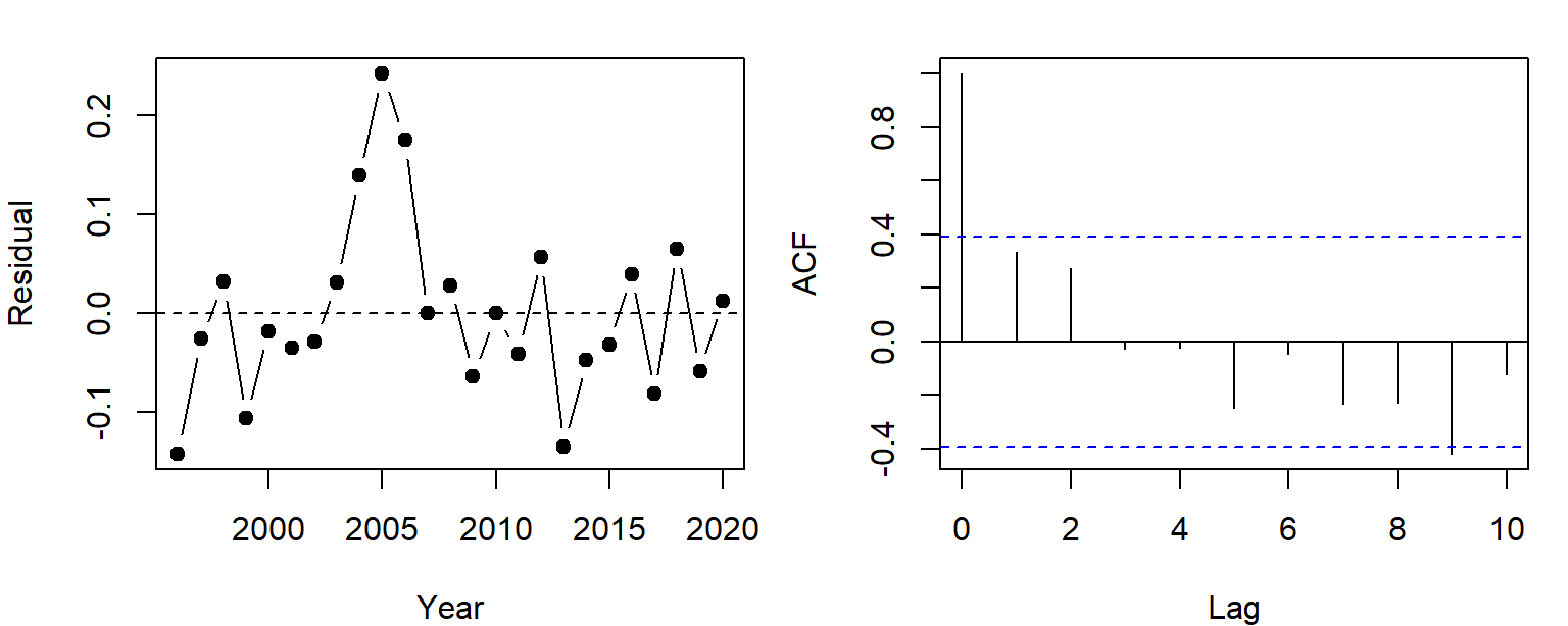

The acf() panel shows the correlation between residuals \(k\) years apart. The lag-1 value, 0.33, falls inside the dashed bounds, so (surprisingly) this plot can't rule out independence. With 25 years the bounds are wide (\(\pm 1.96/\sqrt{25} \approx \pm 0.39\)), and a series this short often hides autocorrelation that's really there.

Other evidence helps. For example, the correlation decays down to zero- a classic sign of serially correlated errors. Also, lag-1 residual correlation is positive in all four stands:

lag1 <- function(dat) {
  dat$year_c <- dat$year - 2008
  acf(resid(lm(width ~ precip + year_c, data = dat)), plot = FALSE)$acf[2]
}
round(sapply(split(chron, chron$stand), lag1), 2)

##    A    B    C    D 
## 0.33 0.33 0.48 0.41

and it's realistic: stored carbohydrates and needles that live several years can lead to the conditions in one year (e.g., a good growth year) bleeding into the next.

The simplest model for temporally correlated errors is the first-order autoregressive model, AR(1): each year's total "error" is a fraction \(\rho\) of last year's plus new noise (often called an 'innovation'),

\[\eta_t = \rho\,\eta_{t-1} + \varepsilon_t, \qquad \varepsilon_t \sim \text{Normal}(0, \sigma^2), \qquad |\rho| < 1\]

Here \(\eta_t\) is the autocorrelated error and \(\varepsilon_t\) is independent noise. Note: many time-series texts (and nlme's output) call the coefficient \(\phi\) rather than \(\rho\).

Taking variances of both sides, with \(\eta_{t-1}\) and \(\varepsilon_t\) independent and \(\text{Var}(\eta_t) = \text{Var}(\eta_{t-1})\) (a stationary series):

\[\text{Var}(\eta_t) = \rho^2\text{Var}(\eta_t) + \sigma^2 \quad\Longrightarrow\quad \text{Var}(\eta_t) = \frac{\sigma^2}{1 - \rho^2}\]

and the correlation between deviations \(k\) steps apart is \(\rho^k\) (Bolker eq. 10.3.7). So the covariance between years \(s\) and \(t\) is

\[V_{st} = \frac{\sigma^2}{1 - \rho^2}\,\rho^{|s - t|}\]

The abs(row(M) - col(M)) trick from Bolker (p. 427) builds the matrix of lags:

lags <- abs(outer(1:25, 1:25, "-"))
V_ar1 <- function(rho, sigma) sigma^2 / (1 - rho^2) * rho^lags
round(V_ar1(0.6, 0.08)[1:5, 1:5], 4)

##        [,1]   [,2]   [,3]   [,4]   [,5]
## [1,] 0.0100 0.0060 0.0036 0.0022 0.0013
## [2,] 0.0060 0.0100 0.0060 0.0036 0.0022
## [3,] 0.0036 0.0060 0.0100 0.0060 0.0036
## [4,] 0.0022 0.0036 0.0060 0.0100 0.0060
## [5,] 0.0013 0.0022 0.0036 0.0060 0.0100

Fitting needs \(|\rho| < 1\), so we optimize \(\text{atanh}(\rho)\), which can be any number, and convert back with tanh(). Standard errors from the Hessian are then on the atanh and log scales; the delta method puts them back into \(\rho\) and \(\sigma\) (see the reference handout The Delta Method).

# mean: a + b * precip + c * year_c; AR(1) errors with rho = tanh(par[4]), sigma = exp(par[5])
nll_ar1 <- function(par) {
  mu <- par[1] + par[2] * chron_a$precip + par[3] * chron_a$year_c
  V <- V_ar1(tanh(par[4]), exp(par[5]))
  -dmvnorm(chron_a$width, mu, V, log = TRUE)
}
fit_ar1 <- optim(c(coef(fit_lm_a), 0, log(0.1)), nll_ar1, method = "BFGS", hessian = TRUE)
c(a = fit_ar1$par[1], b = fit_ar1$par[2], c = fit_ar1$par[3],
  rho = tanh(fit_ar1$par[4]), sigma = exp(fit_ar1$par[5]))

## a.(Intercept)      b.precip      c.year_c           rho         sigma 
##    0.55832666    0.02140853   -0.00467618    0.36721938    0.08181305

library(nlme)
fit_gls <- gls(width ~ precip + year_c, data = chron_a,
               correlation = corAR1(form = ~ year), method = "ML")
coef(fit_gls)

##  (Intercept)       precip       year_c 
##  0.558326882  0.021408527 -0.004676191

coef(fit_gls$modelStruct$corStruct, unconstrained = FALSE)   # rho (nlme calls it Phi)

##       Phi 
## 0.3672189

The estimated \(\rho\) is 0.37. The trend estimate barely moves, but its standard error grows:

• assuming independence: -0.0055 mm/yr, SE 0.0026, \(p =\) 0.045;
• with AR(1) errors: -0.0047 mm/yr, SE 0.0034 (from the Hessian), \(p =\) 0.17.

The simulation has no trend at all.

The widget below builds two covariance structures for 12 observations and simulates data from them. The heatmap shows correlations (blue positive, red negative).

Random intercept (3 groups of 4) AR(1) time series

New random draw

Question: With \(\rho\) near 0.9, what does a single AR(1) series look like? How could you tell it apart from a slow trend?

3. Why these models are harder to fit

The AR(1) model above and the random intercept model for the 20 tree means were both fit with the same optim() call as always:

y_tree <- tree_means$width
Z <- model.matrix(~ 0 + stand, data = tree_means)
V_ri <- function(sigma_b, sigma) sigma_b^2 * Z %*% t(Z) + sigma^2 * diag(20)
nll_ri <- function(par) -dmvnorm(y_tree, rep(par[1], 20), V_ri(exp(par[2]), exp(par[3])), log = TRUE)
fit_ri <- optim(c(mean(y_tree), log(0.1), log(0.1)), nll_ri, method = "BFGS")
sb_hat <- exp(fit_ri$par[2])
s_hat <- exp(fit_ri$par[3])
c(mu = fit_ri$par[1], sigma_b = sb_hat, sigma = s_hat)

##        mu   sigma_b     sigma 
## 1.0312400 0.1419086 0.0847458

Three things make structured-variance models harder than their independent cousins.

Each NLL evaluation costs more. Under independence the NLL is a sum of \(n\) terms. The MVN needs the determinant and inverse of an \(n \times n\) matrix (in practice a Cholesky factorization), which takes on the order of \(n^3\) operations. Doubling the data multiplies the time per evaluation by about 8, and optim() evaluates the NLL hundreds of times.

# milliseconds per NLL evaluation, averaged over 'reps' evaluations
time_nll <- function(n, reps = 10) {
  y <- rnorm(n)
  V <- 0.5^abs(outer(1:n, 1:n, "-"))
  ms <- function(expr) 1000 * system.time(for (i in 1:reps) expr)[["elapsed"]] / reps
  c(n = n, independent = ms(sum(dnorm(y, 0, 1, log = TRUE))),
    mvn = ms(dmvnorm(y, rep(0, n), V, log = TRUE)))
}
set.seed(1)
timings <- t(sapply(c(250, 500, 1000, 2000), time_nll))
timings

##         n independent mvn
## [1,]  250           0   0
## [2,]  500           0   1
## [3,] 1000           0  23
## [4,] 2000           0 153

With 2000 observations, one MVN evaluation took about 153 ms here; the independent NLL took a small fraction of a millisecond. An optim() run needing 300 evaluations would take about 0.8 minutes, against well under a second. (Packages like lme4 and nlme exploit the structure of \(V\), such as its blocks, to avoid most of this cost.)

The likelihood surface is awkward. Below are NLL contours for the two models, with the other parameters set to their best values at each point (a profile). The shaded region is within 1.92 NLL units of the minimum, an approximate 95% confidence region.

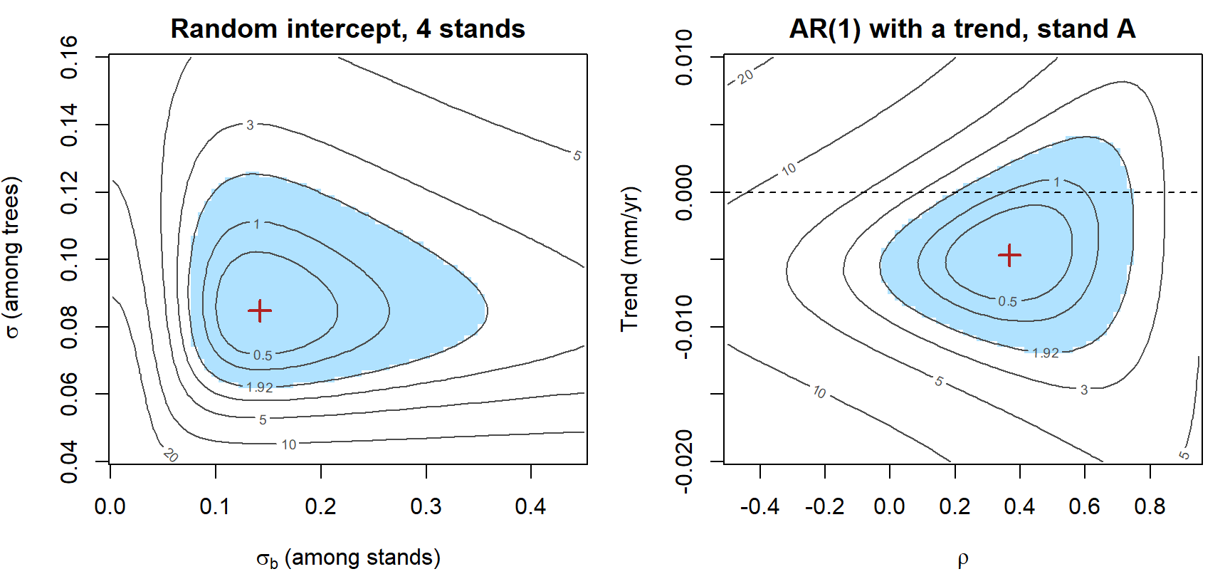
• Random intercept: the region runs from about \(\sigma_b =\) 0.08 to 0.35, more than a fourfold range, while \(\sigma\) (from 20 trees) is much better determined. Four stands give four draws of \(b_j\), so the data say little about their spread. With fewer stands or smaller differences among them, the region reaches \(\sigma_b = 0\); the optimizer may stop on that boundary, where the usual Hessian and LRT approximations fail (the same problem as in comparing Poisson and negative binomial models).
• AR(1) with a trend: here the axes are \(\rho\) and the trend, with everything else profiled out. The region is a fan, not an ellipse. Near \(\rho = 0\) the plausible trends run from about -0.0074 to -0.0039 mm/yr, all below 0 (dashed line). At \(\rho =\) 0.37 they run from -0.0113 to 0.0017. A slow drift and strong autocorrelation can explain the same wandering series, so what we conclude about a mean parameter depends on a variance parameter, and the two have to be estimated together. A lopsided region like this also makes Hessian-based intervals, which assume an ellipse, less trustworthy.

Parameters must keep \(V\) valid. A variance must be positive, \(|\rho|\) must be below 1, and in general \(V\) must stay positive definite. An unconstrained step can leave the allowed region, and dmvnorm() then fails. We avoided this by optimizing \(\log\sigma\) and \(\text{atanh}(\rho)\); richer structures need cleverer parameterizations (for example, building \(V\) from its Cholesky factor, as Stan does in the Bayesian version).

None of this is a reason to assume independence when it's false. It's why specialized software exists for these models, and why Bayesian methods, which sample the random effects instead of integrating over them, are popular for hierarchical models.

4. Random slopes

A new question for a bigger data set: is drought sensitivity the same everywhere? Twelve pinyon stands span an elevation gradient. For each stand we have a ring-width chronology and that stand's winter precipitation, but the records differ in length: two stands have 30 reliable years, two have only 5. (These data are also simulated.) We express precipitation in 10-cm units, centered at 20 cm, so the intercept is the ring width in a 20-cm winter and the slope is the change in width per extra 10 cm.

set.seed(12)
n_years <- rep(c(30, 24, 18, 12, 8, 5), each = 2)        # record length per stand
tau_true <- c(0.15, 0.10)                                 # among-stand SDs: intercept, slope
rho_true <- -0.6
G_true <- diag(tau_true) %*% matrix(c(1, rho_true, rho_true, 1), 2) %*% diag(tau_true)
ab_true <- rmvnorm(12, c(0.9, 0.25), G_true)              # each stand's intercept and slope
stand_names <- sprintf("S%02d", 1:12)
drought <- data.frame(stand = factor(rep(stand_names, n_years)),
                      year = unlist(lapply(n_years, function(n) seq(2021 - n, 2020))))
j <- as.integer(drought$stand)
drought$precip <- round(rgamma(nrow(drought), shape = 9, scale = 22 / 9), 1)
drought$precip10 <- (drought$precip - 20) / 10
drought$width <- round(ab_true[j, 1] + ab_true[j, 2] * drought$precip10 +
                         rnorm(nrow(drought), 0, 0.12), 2)
head(drought)

##   stand year precip precip10 width
## 1   S01 1991   14.1    -0.59  0.36
## 2   S01 1992   18.3    -0.17  0.76
## 3   S01 1993   21.7     0.17  0.69
## 4   S01 1994   21.8     0.18  0.40
## 5   S01 1995   23.4     0.34  0.83
## 6   S01 1996   25.9     0.59  0.97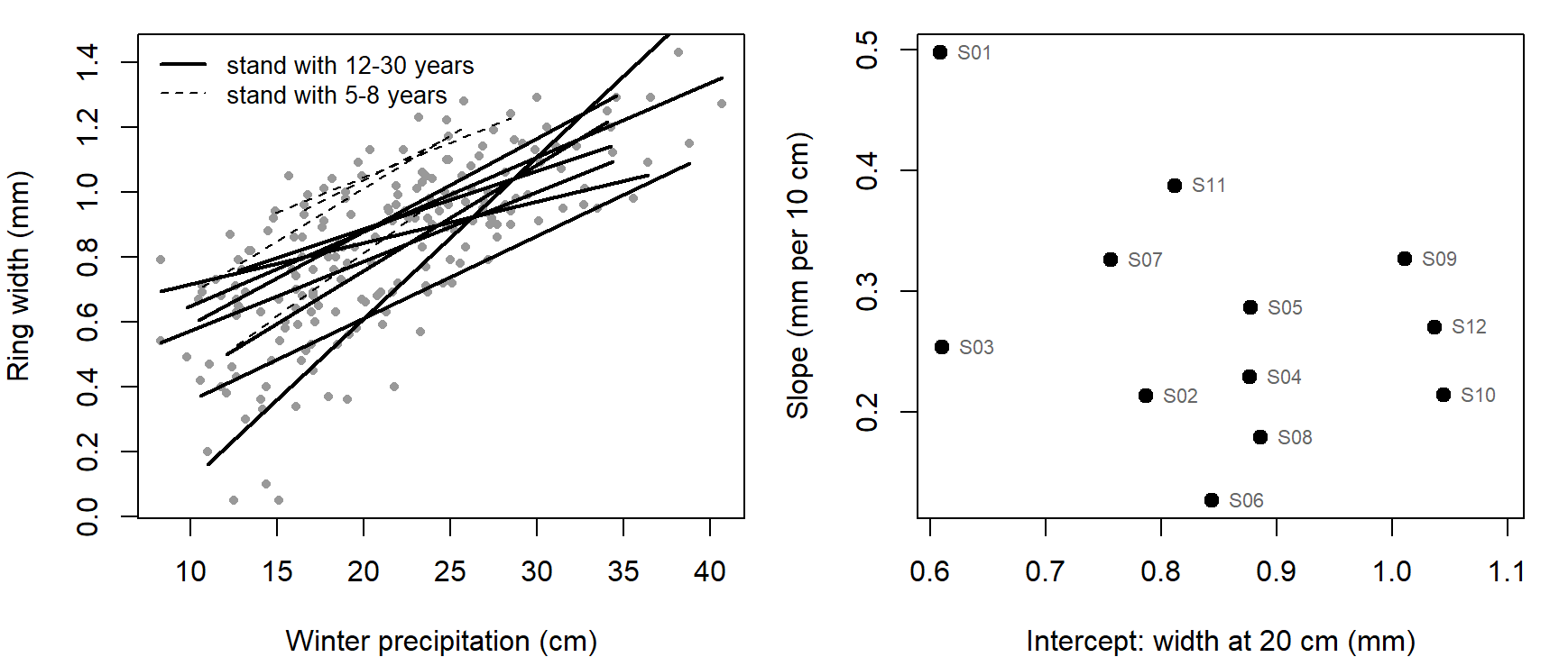

Left: one least-squares line per stand. Right: each stand's own intercept and slope. Stands that grow less in an average winter tend to respond more to precipitation, as you might expect if low-elevation stands are closer to their water limit.

A random slope model lets both the intercept and the slope vary among stands, and lets them be correlated:

\[\text{width}_{jt} = (\mu_a + a_j) + (\mu_b + b_j)\,x_{jt} + \varepsilon_{jt}, \qquad \varepsilon_{jt} \sim \text{Normal}(0, \sigma^2)\]

\[\begin{pmatrix} a_j \\ b_j \end{pmatrix} \sim \text{MVN}\left(\begin{pmatrix} 0 \\ 0 \end{pmatrix}, G\right), \qquad G = \begin{pmatrix} \tau_a^2 & \rho\,\tau_a\tau_b \\ \rho\,\tau_a\tau_b & \tau_b^2 \end{pmatrix}\]

where \(x_{jt}\) is precipitation (10-cm units, centered) for stand \(j\) in year \(t\). There are six parameters: two fixed effects (\(\mu_a\), \(\mu_b\)), the among-stand SDs of the intercepts and slopes (\(\tau_a\), \(\tau_b\)), their correlation \(\rho\), and the residual SD \(\sigma\). The 24 stand deviations \(a_j, b_j\) are not parameters in this likelihood; they're integrated out, just as \(b_j\) was for the random intercept.

What does that do to \(V\)? Within stand \(j\), write the observations as \(y_j = X_j\mu + Z_j u_j + \varepsilon_j\), with \(u_j = (a_j, b_j)^T\) and \(Z_j\) the two-column matrix \([1, x]\) for that stand. Then

\[V_j = Z_j G Z_j^T + \sigma^2 I\]

and \(V\) is block diagonal again, one block per stand, but the covariance between two years in the same stand now depends on how wet those years were.

R's mixed-model packages share a formula syntax for the random part:

Formula	Meaning	Variance parameters
(1 | stand)	an intercept for each stand	1
(precip10 | stand)	an intercept and a slope for each stand, correlated (same as (1 + precip10 | stand))	3
(precip10 || stand)	an intercept and a slope for each stand, uncorrelated	2
(1 | stand/tree)	stand intercepts plus tree-within-stand intercepts (nested)	2
(1 | stand) + (1 | year)	stand intercepts and year intercepts (crossed: every stand is measured in many years)	2

(|| doesn't work as intended with factor predictors in lme4; there the uncorrelated version is written as two separate terms.) Each formula adds the residual variance \(\sigma^2\) on top.

5. Mixed models in R

lme4. lmer() fits Normal mixed models; glmer() fits generalized ones. Here are the random intercept and random slope models for the drought data:

library(lme4)
fit_ri_lmer <- lmer(width ~ precip10 + (1 | stand), data = drought, REML = FALSE)
fit_rs_lmer <- lmer(width ~ precip10 + (precip10 | stand), data = drought, REML = FALSE)
fixef(fit_rs_lmer)

## (Intercept)    precip10 
##   0.8401512   0.2582348

VarCorr(fit_rs_lmer)

##  Groups   Name        Std.Dev. Corr  
##  stand    (Intercept) 0.131469       
##           precip10    0.091688 -0.573
##  Residual             0.118287

AIC(fit_ri_lmer, fit_rs_lmer)

##             df       AIC
## fit_ri_lmer  4 -180.9218
## fit_rs_lmer  6 -216.8994

Letting the slopes vary costs two parameters and lowers AIC by 36. The estimated correlation between stand intercepts and slopes is -0.57. (REML = FALSE gives the plain MLE; by default lmer() uses REML, which corrects the downward bias in variance estimates. Use the MLE when comparing models with different fixed effects by likelihood ratio or AIC.)

nlme and glmmTMB. The same model in two other packages:

fit_rs_lme <- lme(width ~ precip10, random = ~ precip10 | stand, data = drought, method = "ML")

library(glmmTMB)
fit_rs_tmb <- glmmTMB(width ~ precip10 + (precip10 | stand), data = drought)   # ML by default

By hand. The likelihood is a product over stands of MVN densities, one block \(V_j\) each. Building \(G\) from \(\log\tau_a\), \(\log\tau_b\), and \(\text{atanh}(\rho)\) keeps it a valid covariance matrix wherever optim() steps:

rows_by_stand <- split(seq_len(nrow(drought)), drought$stand)
nll_rs <- function(par) {
  tau <- exp(par[3:4])
  rho <- tanh(par[5])
  sigma <- exp(par[6])
  G <- matrix(c(tau[1]^2, rho * tau[1] * tau[2], rho * tau[1] * tau[2], tau[2]^2), 2)
  nll <- 0
  for (rows in rows_by_stand) {
    Zj <- cbind(1, drought$precip10[rows])
    Vj <- Zj %*% G %*% t(Zj) + sigma^2 * diag(length(rows))
    nll <- nll - dmvnorm(drought$width[rows], as.vector(Zj %*% par[1:2]), Vj, log = TRUE)
  }
  nll
}
fit_rs_optim <- optim(c(0.9, 0.25, log(0.1), log(0.1), 0, log(0.1)), nll_rs, method = "BFGS")

tmb_sd <- attr(VarCorr(fit_rs_tmb)$cond$stand, "stddev")
lme_vc <- VarCorr(fit_rs_lme)
compare <- rbind(
  optim = c(fit_rs_optim$par[1:2], exp(fit_rs_optim$par[3:4]), tanh(fit_rs_optim$par[5]),
            exp(fit_rs_optim$par[6]), -fit_rs_optim$value),
  lmer = c(fixef(fit_rs_lmer), vc_rs, logLik(fit_rs_lmer)),
  lme = c(fixef(fit_rs_lme), as.numeric(lme_vc[1:2, "StdDev"]), as.numeric(lme_vc[2, "Corr"]),
          fit_rs_lme$sigma, logLik(fit_rs_lme)),
  glmmTMB = c(fixef(fit_rs_tmb)$cond, tmb_sd,
              attr(VarCorr(fit_rs_tmb)$cond$stand, "correlation")[1, 2],
              sigma(fit_rs_tmb), logLik(fit_rs_tmb)))
colnames(compare) <- c("mu_a", "mu_b", "tau_a", "tau_b", "rho", "sigma", "logLik")
round(compare, 4)

##           mu_a   mu_b  tau_a  tau_b     rho  sigma   logLik
## optim   0.8402 0.2582 0.1315 0.0917 -0.5729 0.1183 114.4497
## lmer    0.8402 0.2582 0.1315 0.0917 -0.5729 0.1183 114.4497
## lme     0.8402 0.2582 0.1315 0.0917 -0.5730 0.1183 114.4497
## glmmTMB 0.8402 0.2582 0.1315 0.0917 -0.5729 0.1183 114.4497

All four agree. The truth is \(\mu_a = 0.9\), \(\mu_b = 0.25\), \(\tau_a = 0.15\), \(\tau_b = 0.10\), \(\rho = -0.6\), \(\sigma = 0.12\).

Which package when:

• lme4 (lmer(), glmer()): fast; handles crossed random effects (stands and years) well. No correlation structures for the residuals.
• nlme (lme(), gls()): residual correlation structures (corAR1(), spatial ones like corExp()) and unequal variances (varIdent(), varPower()). Normal responses only; crossed random effects are awkward.
• glmmTMB: many response distributions (negative binomial, beta, zero-inflated and hurdle models), and covariance structures for the random effects such as ar1() and spatial exp(). It writes the likelihood for you and uses automatic differentiation and the Laplace approximation (see the GLMM bonus).

Question: The estimated correlation between stand intercepts and slopes is -0.57. What does that say about these stands, ecologically? What does it say about a management plan that ranks stands by drought risk using average growth alone?

Discussion

Q1. Switching to AR(1) errors changed the trend's standard error from 0.0026 to 0.0034 mm/yr, but the precipitation slope's from 0.0026 to 0.0020 mm/cm. Why would autocorrelated errors matter more for a trend over time than for precipitation, which jumps around from year to year?

Q2. A colleague says: "I have only four stands, so I'll treat stand as a fixed factor instead of a random intercept." Using the random-intercept surface in section 3, argue for or against. What question is each model answering?

Q3. Fitting the random slope model to only the four short-record stands (S09-S12, 26 stand-years) gives \(\hat\tau_a =\) 0.084, \(\hat\tau_b =\) 0.063, and \(\hat\rho =\) -1.00, with a "boundary (singular) fit" message. Do these stands have perfectly correlated intercepts and slopes? What would you report, and what would you change about the model?

Bonus: a random intercept and AR(1) together

The two structures combine. Using all four pinyon chronologies (100 stand-years), suppose each stand has its own random intercept and AR(1) deviations within the stand:

\[\text{width}_{jt} = a + b_j + \beta\,\text{precip}_t + \eta_{jt}, \qquad b_j \sim \text{Normal}(0, \sigma_b^2), \qquad \eta_{jt} = \rho\,\eta_{j,t-1} + \varepsilon_{jt}\]

\(V\) is the sum of the two pieces: \(\sigma_b^2\) wherever two values share a stand, plus an AR(1) block within each stand. kronecker(A, B) places a copy of B in every cell of A, scaled by that cell, so kronecker(diag(4), B) makes a block-diagonal matrix with four copies of B.

Z_chron <- model.matrix(~ 0 + stand, data = chron)
V_combined <- function(sigma_b, rho, sigma) {
  sigma_b^2 * Z_chron %*% t(Z_chron) + kronecker(diag(4), V_ar1(rho, sigma))
}
nll_combined <- function(par) {
  mu <- par[1] + par[2] * chron$precip
  V <- V_combined(exp(par[3]), tanh(par[4]), exp(par[5]))
  -dmvnorm(chron$width, mu, V, log = TRUE)
}
fit_comb <- optim(c(0.4, 0.02, log(0.1), 0, log(0.1)), nll_combined, method = "BFGS",
                  control = list(maxit = 1000))
c(a = fit_comb$par[1], b = fit_comb$par[2], sigma_b = exp(fit_comb$par[3]),
  rho = tanh(fit_comb$par[4]), sigma = exp(fit_comb$par[5]))

##          a          b    sigma_b        rho      sigma 
## 0.46035584 0.02378212 0.14149076 0.50812194 0.10020520

fit_lme <- lme(width ~ precip, random = ~ 1 | stand, data = chron,
               correlation = corAR1(form = ~ year | stand), method = "ML")
fixef(fit_lme)

## (Intercept)      precip 
##  0.46035191  0.02378214

coef(fit_lme$modelStruct$corStruct, unconstrained = FALSE)

##       Phi 
## 0.5081204

c(-fit_comb$value, logLik(fit_lme))       # same maximized log-likelihood

## [1] 82.27621 82.27621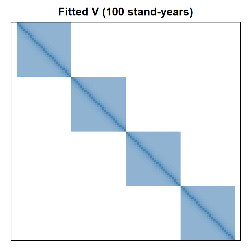

Each block mixes the two structures: correlation decays with the lag between years but levels off at the intraclass correlation instead of reaching 0.

Bonus: a Poisson GLMM by hand

For a count response the random effects can't be integrated out in closed form (see integrating out a random effect). Suppose we counted cones on 8 trees in each of the 12 stands, with tree vigor (standardized) as the predictor:

\[\text{cones}_{ij} \sim \text{Poisson}(\lambda_{ij}), \qquad \log\lambda_{ij} = \beta_0 + \beta_1\,\text{vigor}_{ij} + b_j, \qquad b_j \sim \text{Normal}(0, \sigma_b^2)\]

Each stand's likelihood is a one-dimensional integral over \(b_j\), and integrate() can do it numerically:

set.seed(12)
cones <- data.frame(stand = factor(rep(stand_names, each = 8)),
                    vigor = round(rnorm(96), 2))
b_stand <- rnorm(12, 0, 0.5)
cones$count <- rpois(96, exp(1.5 + 0.4 * cones$vigor + b_stand[as.integer(cones$stand)]))

nll_glmm <- function(par) {
  sigma_b <- exp(par[3])
  nll <- 0
  for (g in split(cones, cones$stand)) {
    # integrand: P(this stand's counts | b) * density of b, for a vector of b values
    stand_lik <- function(b) {
      sapply(b, function(bi) exp(sum(dpois(g$count, exp(par[1] + par[2] * g$vigor + bi), log = TRUE)))) *
        dnorm(b, 0, sigma_b)
    }
    nll <- nll - log(integrate(stand_lik, -Inf, Inf)$value)
  }
  nll
}
fit_glmm <- optim(c(1, 0, log(0.3)), nll_glmm, method = "BFGS")
fit_glmm_tmb <- glmmTMB(count ~ vigor + (1 | stand), family = poisson, data = cones)

rbind(integrate = c(fit_glmm$par[1:2], exp(fit_glmm$par[3]), -fit_glmm$value),
      glmmTMB = c(fixef(fit_glmm_tmb)$cond, attr(VarCorr(fit_glmm_tmb)$cond$stand, "stddev"),
                  logLik(fit_glmm_tmb)))

##           (Intercept)     vigor (Intercept)          
## integrate    1.550849 0.3819203   0.5424088 -225.5694
## glmmTMB      1.548197 0.3820485   0.5422583 -225.5823

The estimates agree to about two decimals; glmmTMB's Laplace approximation is close to the numerical integral here. A random slope would make each stand's integral two-dimensional, and the cost of grid-based integration grows with the number of grid points raised to the number of random effects per group. That's why packages approximate the integral, and why Bayesian samplers, which skip it, are popular for complex hierarchical models.

Bayesian hierarchical models

The same random slope model, fit by MCMC. A Bayesian hierarchical model puts priors on the population-level parameters (the among-stand SDs and the correlation), and the sampler draws each stand's intercept and slope along with everything else. This part covers partial pooling, priors for a covariance matrix, the model written in Stan, and the same model in one line of brms.

1. Big picture

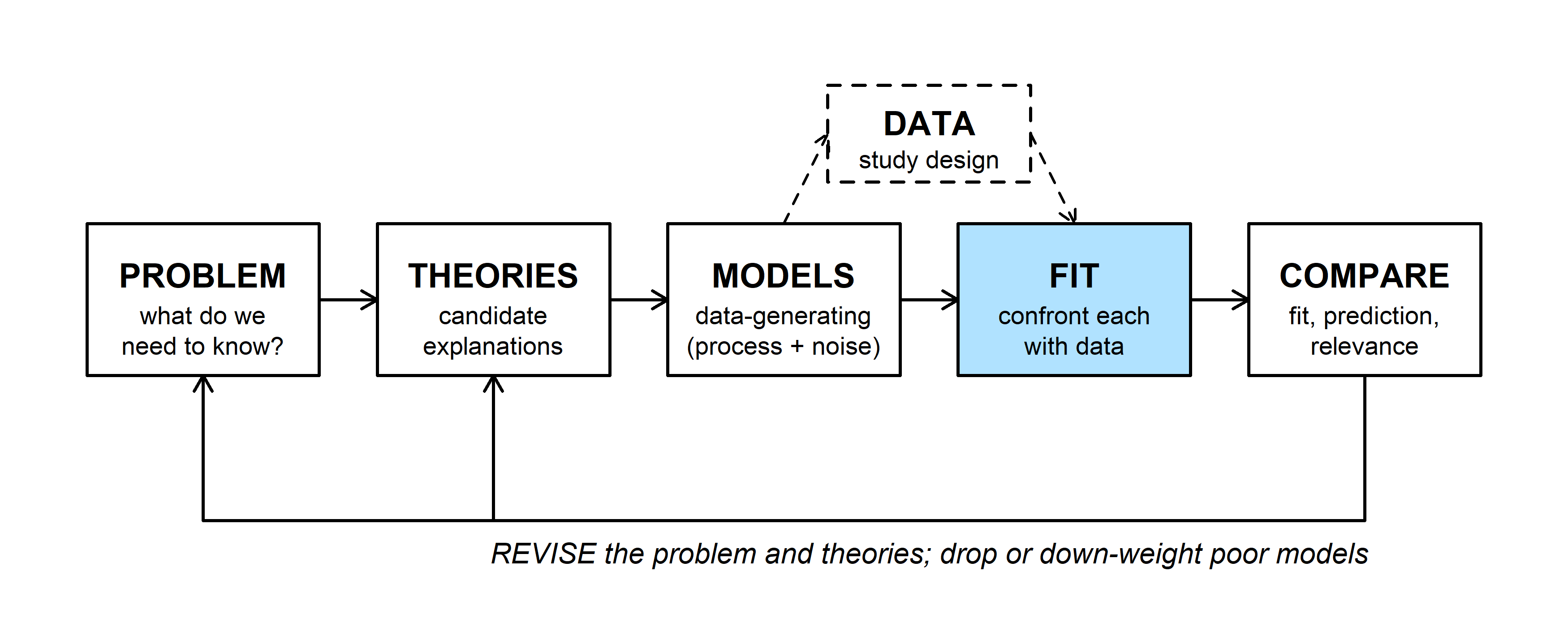
"Hierarchical," "multilevel," and "mixed" describe the same models. In Bayesian terms, a random effect is a parameter whose prior has its own unknown parameters (hyperparameters): each \((a_j, b_j)\) gets the prior \(\text{MVN}(0, G)\), and \(G\) gets a prior too. Compared with fitting by maximum likelihood:

• No integral. The sampler draws the \(a_j\) and \(b_j\) instead of integrating them out, so a Poisson or binomial response is no harder than a Normal one.
• Uncertainty carries through. Each stand's estimate reflects uncertainty in \(\tau_a\), \(\tau_b\), and \(\rho\), rather than plugging in their best values.
• Priors help with few groups. A weakly informative prior keeps an SD off the boundary at 0 and a correlation off \(\pm 1\), where maximum likelihood gave up in Q3.
• The price is choosing priors and checking the sampler (see checking chains).

2. Partial pooling

There are three ways to estimate each stand's mean ring width:

• complete pooling: ignore stands; every stand gets the overall mean;
• no pooling: estimate each stand separately (stand as a fixed factor);
• partial pooling: the random effect, a compromise between the two.

Ignoring precipitation for the moment, a random intercept model gives stand \(j\) the estimate

\[\hat a_j = \hat\mu + w_j(\bar y_j - \hat\mu), \qquad w_j = \frac{\sigma_b^2}{\sigma_b^2 + \sigma^2/n_j}\]

where \(\bar y_j\) is the stand's own mean from \(n_j\) years. The weight \(w_j\) compares the spread among stands (\(\sigma_b^2\)) with the sampling variance of the stand's own mean (\(\sigma^2/n_j\)). A stand with a long record keeps most of its own mean; a stand with 5 years is pulled toward the overall mean. This is the same precision-weighted average as a Normal prior combined with Normal data (priors and posteriors): the population of stands acts as a prior for each stand.

fit_ri0 <- lmer(width ~ 1 + (1 | stand), data = drought, REML = FALSE)
sd_ri0 <- as.data.frame(VarCorr(fit_ri0))$sdcor          # sigma_b, sigma
ybar <- tapply(drought$width, drought$stand, mean)
n_j <- as.vector(table(drought$stand))
w <- sd_ri0[1]^2 / (sd_ri0[1]^2 + sd_ri0[2]^2 / n_j)
round(cbind(own_mean = ybar, n_j, w, formula = fixef(fit_ri0) + w * (ybar - fixef(fit_ri0)),
            lmer = coef(fit_ri0)$stand[, 1]), 3)

##     own_mean n_j     w formula  lmer
## S01    0.704  30 0.879   0.723 0.723
## S02    0.838  30 0.879   0.841 0.841
## S03    0.593  24 0.853   0.633 0.633
## S04    0.911  24 0.853   0.904 0.904
## S05    0.881  18 0.814   0.877 0.877
## S06    0.867  18 0.814   0.866 0.866
## S07    0.895  12 0.744   0.886 0.886
## S08    0.916  12 0.744   0.902 0.902
## S09    0.955   8 0.660   0.923 0.923
## S10    1.090   8 0.660   1.012 1.012
## S11    0.772   5 0.548   0.812 0.812
## S12    1.038   5 0.548   0.958 0.958

The formula matches lmer()'s stand estimates. Here \(\hat\sigma_b =\) 0.113 and \(\hat\sigma =\) 0.229; the widget starts at those values. It plots each stand's own mean and its partially pooled estimate.

Among-stand SD σ_b

Within-stand SD σ

Weight on own mean, 30 years

Weight on own mean, 5 years

Overall mean μ̂

Open circles: each stand's own mean (no pooling). Filled circles: partially pooled estimates. Dashed line: the overall mean (complete pooling).

Question: Set \(\sigma_b\) to 0, then drag it to 0.4. Which two pooling choices are these? Then compare S10 and S12: their own means are similar (1.09 and 1.04), but one has 8 years and the other 5. Which moves more toward the overall mean, and why?

3. Priors for a covariance matrix

The random slope model needs a prior on \(G\), a 2 \(\times\) 2 covariance matrix. The usual approach splits \(G\) into scales and correlations,

\[G = \begin{pmatrix} \tau_a & 0 \\ 0 & \tau_b \end{pmatrix} \Omega \begin{pmatrix} \tau_a & 0 \\ 0 & \tau_b \end{pmatrix}, \qquad \Omega = \begin{pmatrix} 1 & \rho \\ \rho & 1 \end{pmatrix}\]

and puts separate priors on each piece: a half-Normal, half-\(t\), or exponential prior on each SD \(\tau\), and an LKJ prior on the correlation matrix \(\Omega\) (named for Lewandowski, Kurowicka, and Joe). Older BUGS and JAGS code often used an inverse-Wishart prior on \(G\) instead, which ties the prior on the SDs to the prior on the correlations; splitting them makes each easier to choose.

The LKJ density has one shape parameter \(\eta\):

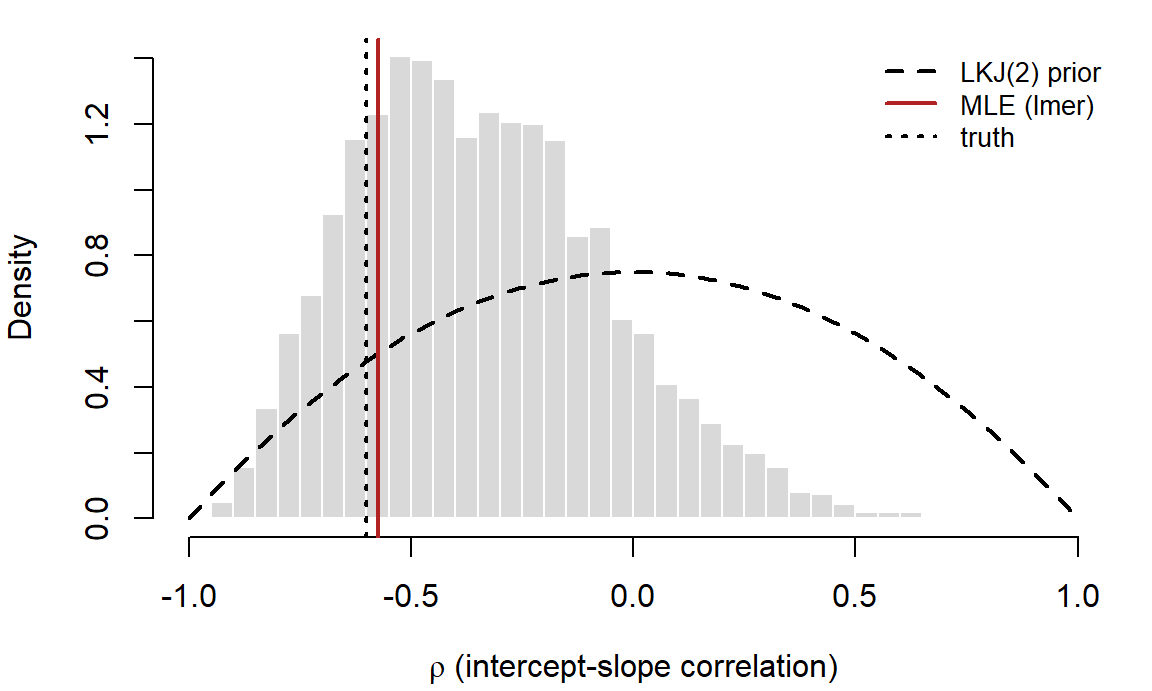
\[p(\Omega) \propto \det(\Omega)^{\eta - 1}\]

For a 2 \(\times\) 2 matrix, \(\det(\Omega) = 1 - \rho^2\), so \(p(\rho) \propto (1 - \rho^2)^{\eta - 1}\). With \(\eta = 1\) every correlation is equally likely; \(\eta > 1\) favors correlations near 0, and \(\eta < 1\) favors correlations near \(\pm 1\). For a bigger matrix (\(K \times K\)), each single correlation has the marginal prior \((\rho + 1)/2 \sim \text{Beta}(\eta - 1 + K/2,\ \eta - 1 + K/2)\).

Size of the correlation matrix: 2 × 2 (intercept, slope) 4 × 4 10 × 10

Shape η

Prior P(|ρ| > 0.5)

Prior P(|ρ| > 0.8)

Prior SD of ρ

Question: For a 10 \(\times\) 10 correlation matrix with \(\eta = 1\), how likely is any one correlation to exceed 0.5 in absolute value? What does "uniform" mean for a matrix that large?

4. Random slopes in Stan

The Stan program below is the random slope model with an LKJ(2) prior on \(\Omega\). Two choices in it need explaining.

• The Cholesky factor. Stan works with \(L\), the lower-triangular matrix with \(LL^T = \Omega\). Any value Stan proposes for cholesky_factor_corr gives a valid correlation matrix, so the sampler can't leave the allowed region (the third problem in why these models are harder to fit), and it's cheaper to compute with.
• Non-centered stand effects. Instead of sampling \((a_j, b_j)\) directly, Stan samples standard Normal \(z_j\) and computes \((a_j, b_j)^T = \text{diag}(\tau)\,L\,z_j\). This avoids the funnel that makes hierarchical models hard to sample (when HMC struggles).

library(cmdstanr)
slopes_code <- "
data {
  int<lower=1> N;                       // stand-years
  int<lower=1> J;                       // stands
  array[N] int<lower=1, upper=J> stand;
  vector[N] x;                          // precipitation (10 cm, centered at 20 cm)
  vector[N] y;                          // ring width (mm)
}
parameters {
  vector[2] mu;                         // mean intercept and slope
  vector<lower=0>[2] tau;               // among-stand SDs of intercepts and slopes
  cholesky_factor_corr[2] L;            // Cholesky factor of the correlation matrix
  matrix[2, J] z;                       // standardized stand effects
  real<lower=0> sigma;                  // residual SD
}
transformed parameters {
  // row j: stand j's intercept and slope
  matrix[J, 2] ab = rep_matrix(mu', J) + (diag_pre_multiply(tau, L) * z)';
}
model {
  mu[1] ~ normal(1, 0.5);
  mu[2] ~ normal(0, 0.5);
  tau ~ normal(0, 0.3);                 // half-normal, because tau > 0
  L ~ lkj_corr_cholesky(2);
  to_vector(z) ~ std_normal();
  sigma ~ normal(0, 0.3);
  y ~ normal(ab[stand, 1] + ab[stand, 2] .* x, sigma);
}
generated quantities {
  real rho = multiply_lower_tri_self_transpose(L)[1, 2];
}
"
slopes_model <- cmdstan_model(write_stan_file(slopes_code))
stan_data <- list(N = nrow(drought), J = 12, stand = as.integer(drought$stand),
                  x = drought$precip10, y = drought$width)
fit_stan <- slopes_model$sample(data = stan_data, chains = 4, parallel_chains = 4,
                                seed = 746, refresh = 0)

Check the sampler first, then the estimates:

fit_stan$diagnostic_summary()

## $num_divergent
## [1] 0 0 0 0
## 
## $num_max_treedepth
## [1] 0 0 0 0
## 
## $ebfmi
## [1] 0.7179343 0.6909448 0.6911174 0.7042722

fit_stan$summary(c("mu", "tau", "rho", "sigma"))

## # A tibble: 6 × 10
##   variable   mean median      sd     mad      q5   q95  rhat ess_bulk ess_tail
##   <chr>     <dbl>  <dbl>   <dbl>   <dbl>   <dbl> <dbl> <dbl>    <dbl>    <dbl>
## 1 mu[1]     0.842  0.842 0.0468  0.0441   0.765  0.920  1.00     834.    1263.
## 2 mu[2]     0.263  0.263 0.0382  0.0362   0.200  0.324  1.00    1421.    1725.
## 3 tau[1]    0.154  0.149 0.0377  0.0344   0.103  0.224  1.00    1233.    1852.
## 4 tau[2]    0.111  0.106 0.0317  0.0283   0.0688 0.170  1.00    1748.    2165.
## 5 rho      -0.341 -0.366 0.282   0.292   -0.756  0.172  1.00    2259.    2415.
## 6 sigma     0.119  0.119 0.00664 0.00653  0.109  0.131  1.00    4092.    2598.

Maximum likelihood (lmer) and posterior summaries

	truth	lmer	posterior median	5%	95%
mu_a	0.90	0.840	0.842	0.765	0.920
mu_b	0.25	0.258	0.263	0.200	0.324
tau_a	0.15	0.131	0.149	0.103	0.224
tau_b	0.10	0.092	0.106	0.069	0.170
rho	-0.60	-0.573	-0.366	-0.756	0.172
sigma	0.12	0.118	0.119	0.109	0.131

The two methods agree closely on everything except the correlation: the MLE is -0.57, while the posterior median is -0.37 with a 90% interval from -0.76 to 0.17.

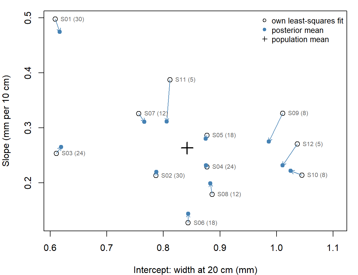
Each arrow runs from a stand's own fit to its posterior mean; the number in parentheses is the record length. Stands with short records move the most; stands with 24 or 30 years barely move.

Because the data are simulated, we can compare both sets of estimates with the true stand values. For the four stands with 5 or 8 years, the average error in the slopes is 0.057 mm per 10 cm with no pooling and 0.055 with partial pooling (intercepts: 0.044 and 0.053 mm). That's a mixed result: in any one data set, shrinkage can pull a stand that really is unusual too far toward the mean. Its advantage is on average. Over 500 simulated data sets with the same design, using lmer()'s stand estimates, partial pooling cut the average slope error for the short-record stands from 0.070 to 0.051 (intercepts: 0.044 to 0.041).

Question: Why is the posterior for \(\rho\) so much wider than the other posteriors, and why is its median closer to 0 than the MLE? Which summary is more honest about what 12 stands can tell us?

Question: Change lkj_corr_cholesky(2) to lkj_corr_cholesky(1), then to lkj_corr_cholesky(10), and refit. Predict how the posterior for \(\rho\) will move before you run each one. Do the stand estimates change much?

5. The same model in brms

brms writes the Stan program from a lme4-style formula. Here are the same model and priors (the fixed-effect priors are left at brms's defaults):

library(brms)
fit_brms <- brm(width ~ precip10 + (precip10 | stand), data = drought,
                prior = c(prior(normal(0, 0.3), class = sd),
                          prior(lkj(2), class = cor),
                          prior(normal(0, 0.3), class = sigma)),
                backend = "cmdstanr", chains = 4, cores = 4, seed = 746, refresh = 0)

summary(fit_brms)

##  Family: gaussian 
##   Links: mu = identity; sigma = identity 
## Formula: width ~ precip10 + (precip10 | stand) 
##    Data: drought (Number of observations: 194) 
##   Draws: 4 chains, each with iter = 2000; warmup = 1000; thin = 1;
##          total post-warmup draws = 4000
## 
## Multilevel Hyperparameters:
## ~stand (Number of levels: 12) 
##                         Estimate Est.Error l-95% CI u-95% CI Rhat Bulk_ESS
## sd(Intercept)               0.16      0.04     0.10     0.25 1.00     1183
## sd(precip10)                0.11      0.03     0.06     0.18 1.00     1426
## cor(Intercept,precip10)    -0.33      0.29    -0.81     0.30 1.00     2170
##                         Tail_ESS
## sd(Intercept)               2170
## sd(precip10)                2371
## cor(Intercept,precip10)     2652
## 
## Regression Coefficients:
##           Estimate Est.Error l-95% CI u-95% CI Rhat Bulk_ESS Tail_ESS
## Intercept     0.84      0.05     0.76     0.93 1.00     1045     1394
## precip10      0.27      0.04     0.19     0.34 1.00     1712     2016
## 
## Further Distributional Parameters:
##       Estimate Est.Error l-95% CI u-95% CI Rhat Bulk_ESS Tail_ESS
## sigma     0.12      0.01     0.11     0.13 1.00     3832     2827
## 
## Draws were sampled using sample(hmc). For each parameter, Bulk_ESS
## and Tail_ESS are effective sample size measures, and Rhat is the potential
## scale reduction factor on split chains (at convergence, Rhat = 1).

The estimates match the hand-written model up to Monte Carlo error. stancode(fit_brms) prints the Stan program brms wrote; it uses the same Cholesky factor and non-centered stand effects. Without the prior argument, brms uses an LKJ(1) prior on the correlations and half-Student-\(t\) priors on the SDs; prior_summary(fit_brms) lists every prior in a fit. rstanarm::stan_lmer() fits the same formula from precompiled models, so it skips the compile step.

Discussion

Q1. With 12 stands, the 90% interval for \(\rho\) runs from -0.76 to 0.17. To rule out \(\rho = 0\), would you rather have 12 more stands or 20 more years at each of the 12 stands? Defend your choice.

Q2. When would you use brms, and when would you write the Stan model yourself?

Q3. Do your final project data have groups (sites, individuals, years, observers)? Which effects would you treat as random, and would you let any slopes vary among groups?

Bonus: ridge regression as a prior

A ridge penalty adds \(\lambda\sum\beta_k^2\) to the NLL. A Normal(0, \(\tau^2\)) prior on each \(\beta_k\) adds \(-\log p(\beta) = \sum\beta_k^2/(2\tau^2)\) plus a constant, which is the same penalty with \(\lambda = 1/(2\tau^2)\); a Laplace prior gives the lasso (see Bayesian model comparison and shrinkage priors). A random effect does the same thing to the stand deviations: the \(\text{MVN}(0, G)\) prior shrinks every \((a_j, b_j)\) toward 0. The difference is that \(\tau\) isn't chosen by cross-validation; it's estimated from how much the stands actually differ.