NRES 746 Code Demo
Emily Ferrell and Joe Coolidge
2025-10-21
click here for the R code for this lecture
Multi-Level (Hierarchical) Regression
Today we will be discussing when, why, and how to use Multi-level (mixed effects) models in R with the packages ‘lme4’ and ‘glmmTMB’.
These are frequentist tools for extensions of simple linear regression.
Let’s ground ourselves with this simple formula for linear regression
where y is our response variable, x is our predictor variable, b0 is our intercept term, b1 is our slope term, and we have some error term epsilon. \[y = \beta_0 + \beta_1*x_1 + \epsilon\] We can also include multiple predictor variables. \[y = \beta_0 + \beta_1*x_1 + \beta_2*x_2+ ...+\beta_n*x_n +\epsilon\] And include interaction terms between multiple predictors. \[y = \beta_0 + \beta_1*x_1 + \beta_2*x_2+ \beta_3*(x_1*x_2) +\epsilon\] We will continue to build off this formula.
Now we need to make sure all of our packages are loaded. Here are the ones you will need:
#install.packages("lme4")
#install.packages("glmmTMB")
#install.packages("ggplot2")
#install.packages("broom.mixed")
#install.packages("performance")
#install.packages("DHARMa")
#install.packages("effects")
Next we will get our data.
This is some data on juvenile owl begging calls that is included in the glmmTMB package.
library(glmmTMB)
data("Owls")
head(Owls)
## Nest FoodTreatment SexParent ArrivalTime SiblingNegotiation BroodSize
## 1 AutavauxTV Deprived Male 22.25 4 5
## 2 AutavauxTV Satiated Male 22.38 0 5
## 3 AutavauxTV Deprived Male 22.53 2 5
## 4 AutavauxTV Deprived Male 22.56 2 5
## 5 AutavauxTV Deprived Male 22.61 2 5
## 6 AutavauxTV Deprived Male 22.65 2 5
## NegPerChick logBroodSize
## 1 0.8 1.609438
## 2 0.0 1.609438
## 3 0.4 1.609438
## 4 0.4 1.609438
## 5 0.4 1.609438
## 6 0.4 1.609438Key variables we will use:
- SiblingNegotiation (count of begging calls)
- FoodTreatment (deprived vs satiated)
- SexParent (female/male)
- Nest
SiblingNegotiation will be our response variable, and FoodTreatment and SexParent are predictor variables. We could draft a simple model where \[SiblingNegotiation = \beta_0 + \beta_1*(FoodTreatment) + \beta_2*(SexParent) + \epsilon\] Or include an interaction term between our predictors. \[SiblingNegotiation = \beta_0 + \beta_1*(FoodTreatment) + \beta_2*(SexParent) + \beta_3*(FoodTreatment*SexParent) + \epsilon\] But what about our nest variable?
That is where mixed effects models come in!!
How do we know a multi-level mixed effects model is the right choice?
Hierarchical models combine fixed effects with random effects. When you have data with some sort of grouping, repetition, or hierarchical structure (e.g., site, plot, nest, year, individual) with repeated measurements this is the right model for you.
Observations within the same group are not independent. In other words, differences in our response variable can be partially explained by group identity. Mixed models explicitly account for that by allowing each group (nest, plot, etc.) to have its own random intercept or slope.
In this case, nest is our grouping factor with repeated measurements or visits to the same owl nest. So, we will treat nest as a random effect in our multi-level mixed effects models.
Lets visualize our data!
library(ggplot2)

ggplot(Owls, aes(SiblingNegotiation)) +
       geom_histogram(binwidth = 1) +
       labs(title = "Begging calls per visit", x = "Calls", y = "Frequency")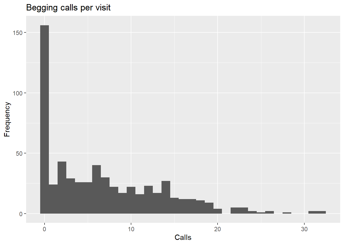
Already, it is clear that we are not dealing with a normally distributed response variable (this is common!). For the purpose of this demo, we will subset out the zeros (don’t worry we will come back to them).
owldata <- subset(Owls, SiblingNegotiation > 0) # remove zeros
summary(owldata$SiblingNegotiation) # double check distribution
## Min. 1st Qu. Median Mean 3rd Qu. Max.
## 1.000 4.000 8.000 9.086 13.000 32.000ggplot(owldata, aes(SiblingNegotiation)) +
geom_histogram(binwidth = 1) +
labs(title = "Begging calls per visit", x = "Calls", y = "Frequency")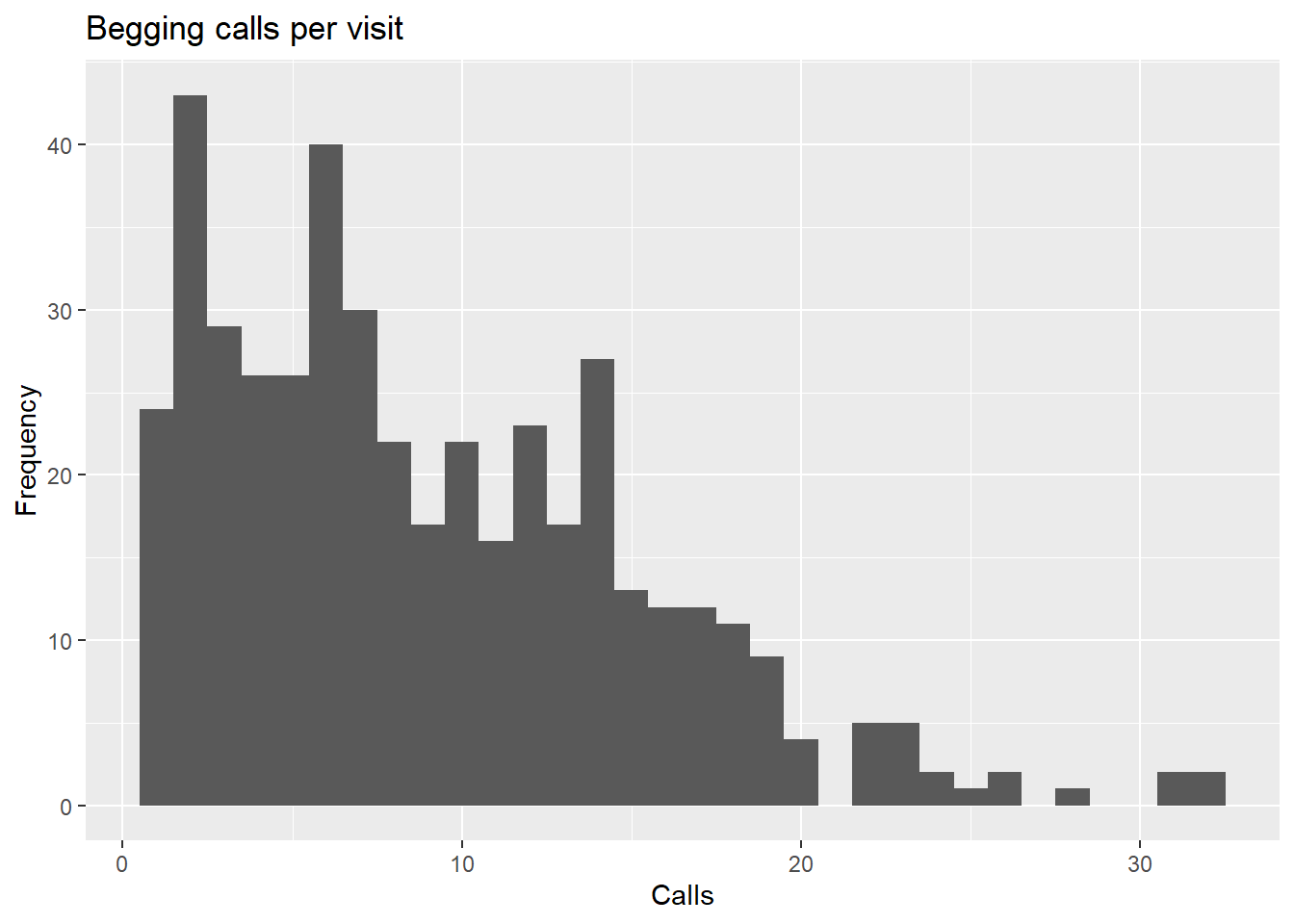
The data is still not normally distributed. It is right skewed, which is pretty typical when you are looking at count data from discrete events (like bird calls).
That this is count data narrows things down to a couple potential distributions: Poisson or negative binomial.
A Poisson distribution has mean equal to variance . \[E[Y] = \lambda, Var[Y] = \lambda\] Whereas a negative binomial distribution has an additional dispersion parameter such that variance can be greater than the mean. \[E[Y] = \mu, Var[Y] = \mu + (\mu^2/\theta)\] Let’s check how the variance in our data compares to the mean.
var(owldata$SiblingNegotiation) # Var(Y)## [1] 38.65778mean(owldata$SiblingNegotiation) # E(Y)## [1] 9.085779Clearly the observed variability is much greater than the expected. In this case, we can use a mixed-effects model with a negative binomial distribution to fit our data! The negative binomial introduces an extra dispersion parameter that allows variance to grow faster than the mean.
Multi-level (mixed effects) models
We want to analyze the effect of the experimental treatment and sex of the parent bringing food on the number of calls (SiblingNegotiation) with a random effect of nest:
\[SiblingNegotiation = \beta_0 + \beta_1*(FoodTreatment) + \beta_2*(SexParent) + \beta_3*(FoodTreatment*SexParent) + \epsilon_{Nest} + \epsilon\] \[ \text{SiblingNegotiation} \sim \text{NegBinomial}(\mu, \theta) \]
Lets start with the package “lme4”
library(lme4)## Loading required package: MatrixWithin this package, there are many functions for modeling mixed-effects models. Here are some of the most common ones:
- glmer() fits GLMMs
- glmer.nb() fits negative binomial GLMMs
- lmer() fits linear mixed-effects models
- nlmer() fits nonlinear mixed-effects models
We will be using glmer.nb() to fit our model.
owls_lme4_nb <- glmer.nb(
SiblingNegotiation ~ FoodTreatment * SexParent # This is shorthand for each predictor and the interaction between both

+ (1|Nest), # This is the syntax for including Nest as a random effect
data = owldata
)
summary(owls_lme4_nb)
## Generalized linear mixed model fit by maximum likelihood (Laplace
## Approximation) [glmerMod]
## Family: Negative Binomial(2.9031) ( log )
## Formula: SiblingNegotiation ~ FoodTreatment * SexParent + (1 | Nest)
## Data: owldata
##
## AIC BIC logLik -2*log(L) df.resid
## 2763.2 2787.7 -1375.6 2751.2 437
##
## Scaled residuals:
## Min 1Q Median 3Q Max
## -1.3622 -0.7957 -0.1403 0.6086 3.9389
##
## Random effects:
## Groups Name Variance Std.Dev.
## Nest (Intercept) 0.03408 0.1846
## Number of obs: 443, groups: Nest, 27
##
## Fixed effects:
## Estimate Std. Error z value Pr(>|z|)
## (Intercept) 2.227067 0.080504 27.664 <2e-16 ***
## FoodTreatmentSatiated -0.179661 0.116361 -1.544 0.123
## SexParentMale -0.011525 0.092161 -0.125 0.900
## FoodTreatmentSatiated:SexParentMale 0.008791 0.143165 0.061 0.951
## ---
## Signif. codes: 0 '***' 0.001 '**' 0.01 '*' 0.05 '.' 0.1 ' ' 1
##
## Correlation of Fixed Effects:
## (Intr) FdTrtS SxPrnM
## FdTrtmntStt -0.557
## SexParentMl -0.704 0.532
## FdTrtmS:SPM 0.441 -0.778 -0.632Note that glmer.nb() automatically uses a log link function
Takeaways
- Random effects: there is relatively little variability between nests (Std. Dev. = 0.1846)
- Fixed effects: no meaningful effects of or interactions between FoodTreatment and SexParent (p >> 0.05)
This model is rather uninformative, but is it misspecified? Let’s dive into some diagnostic tools to check.
The “DHARMa” package is a great way to get diagnostics plots when running mixed-effects models.
library(DHARMa)## This is DHARMa 0.4.7. For overview type '?DHARMa'. For recent changes, type news(package = 'DHARMa')par(mfrow = c(2, 2))
res <- simulateResiduals(owls_lme4_nb, plot = FALSE)
plot(res)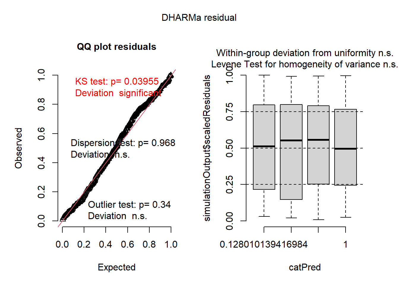
Based on these plots, the model fits very well!
QQ Plot
- shows generally good fit in the residual distribution
- negative binomial family captures variance structure
- no problematic outliers
Residuals by Predicted Bins
- shows no heteroscedasticity and no systematic pattern in residuals vs fitted values
So, the model is a good fit to the data (correctly specified), it’s just not very informative (our predictors don’t have “significant” effects). Maybe that’s because we removed a large portion of the data…
Evaluate performance of the model
library(broom.mixed)
library(performance)
tidy(owls_lme4_nb, effects = "fixed", conf.int = TRUE)## # A tibble: 4 × 8
## effect term estimate std.error statistic p.value conf.low conf.high
## <chr> <chr> <dbl> <dbl> <dbl> <dbl> <dbl> <dbl>
## 1 fixed (Intercept) 2.23 0.0805 27.7 1.88e-168 2.07 2.38
## 2 fixed FoodTreatmen… -0.180 0.116 -1.54 1.23e- 1 -0.408 0.0484
## 3 fixed SexParentMale -0.0115 0.0922 -0.125 9.00e- 1 -0.192 0.169
## 4 fixed FoodTreatmen… 0.00879 0.143 0.0614 9.51e- 1 -0.272 0.289Based on the model, there is no strong evidence that either food treatment or parent sex meaningfully changes the rate of begging calls in this filtered (non-zero) dataset.
r2_nakagawa(owls_lme4_nb)## # R2 for Mixed Models
##
## Conditional R2: 0.099
## Marginal R2: 0.017Marginal \(R^2\)
- this value shows that the fixed predictors (FoodTreatment, SexParent, interaction) explain very little of the total variance in begging calls
- this is consistent with the non-significant outputs above
Conditional \(R^2\)
- the increase in this value indicates that most of the explained variation comes from nest-to-nest differences
Now lets try the package “glmmTMB”
This package is much more model-specific than “lme4” and fits linear and generalized linear mixed models using Template Model Builder for Maximum Likelihood Estimates. The “glmmTMB” package is usually a better fit for ‘weird’ data, such as zero-inflated data.
Remember that lme4 has different functions for different distributions:
- lmer() –> Gaussian (normal)
- glmer() –> any standard GLM family
- glmer.nb() –> wrapper for glmer() that allows it to fit a negative binomial model
However, glmmTMB is much more flexible (at the sacrifice of longer run times). glmmTMB has more options to specify distribution family (including 2 types of negative binomial distributions), and it has options to specify a zero-inflation model or dispersion model! It can even handle hurdle models, but we won’t steal Ryan and Catherine’s thunder…
First, let’s compare nbinom1 and nbinom2. Both handle overdispersion by including an additional dispersion parameter (compared to a Poisson distribution where mean = variance)
nbinom1 has the following variance formula: \[Var = \mu * (1+\alpha)\] And is useful for mild overdispersion.
nbinom2 has the following variance formula: \[Var = \mu + (\mu^2/\theta)\] And is useful for strong overdispersion.
Let’s see how it works on our subsetted data…
library(glmmTMB)
owls_tmb_nb1 <- glmmTMB(
SiblingNegotiation ~ FoodTreatment * SexParent + (1|Nest),
data = owldata,
family = nbinom1()
)
summary(owls_tmb_nb1)
## Family: nbinom1 ( log )
## Formula: SiblingNegotiation ~ FoodTreatment * SexParent + (1 | Nest)
## Data: owldata
##
## AIC BIC logLik -2*log(L) df.resid
## 2760.3 2784.9 -1374.2 2748.3 437
##
## Random effects:
##
## Conditional model:
## Groups Name Variance Std.Dev.
## Nest (Intercept) 0.02758 0.1661
## Number of obs: 443, groups: Nest, 27
##
## Dispersion parameter for nbinom1 family (): 3.1
##
## Conditional model:
## Estimate Std. Error z value Pr(>|z|)
## (Intercept) 2.25461 0.07534 29.924 <2e-16 ***
## FoodTreatmentSatiated -0.22612 0.11171 -2.024 0.0429 *
## SexParentMale -0.01843 0.08586 -0.215 0.8300
## FoodTreatmentSatiated:SexParentMale 0.03472 0.13719 0.253 0.8002
## ---
## Signif. codes: 0 '***' 0.001 '**' 0.01 '*' 0.05 '.' 0.1 ' ' 1owls_tmb_nb2 <- glmmTMB(
SiblingNegotiation ~ FoodTreatment * SexParent + (1|Nest),
data = owldata,
family = nbinom2()
)
summary(owls_tmb_nb2)## Family: nbinom2 ( log )
## Formula: SiblingNegotiation ~ FoodTreatment * SexParent + (1 | Nest)
## Data: owldata
##
## AIC BIC logLik -2*log(L) df.resid
## 2763.0 2787.6 -1375.5 2751.0 437
##
## Random effects:
##
## Conditional model:
## Groups Name Variance Std.Dev.
## Nest (Intercept) 0.03459 0.186
## Number of obs: 443, groups: Nest, 27
##
## Dispersion parameter for nbinom2 family (): 2.9
##
## Conditional model:
## Estimate Std. Error z value Pr(>|z|)
## (Intercept) 2.233082 0.080856 27.618 <2e-16 ***
## FoodTreatmentSatiated -0.180771 0.116696 -1.549 0.121
## SexParentMale -0.012153 0.092409 -0.132 0.895
## FoodTreatmentSatiated:SexParentMale 0.009574 0.143447 0.067 0.947
## ---
## Signif. codes: 0 '***' 0.001 '**' 0.01 '*' 0.05 '.' 0.1 ' ' 1Now we can run our diagnostics plots
res_tmb1  <- simulateResiduals(owls_tmb_nb1, plot = FALSE)
plot(res_tmb1)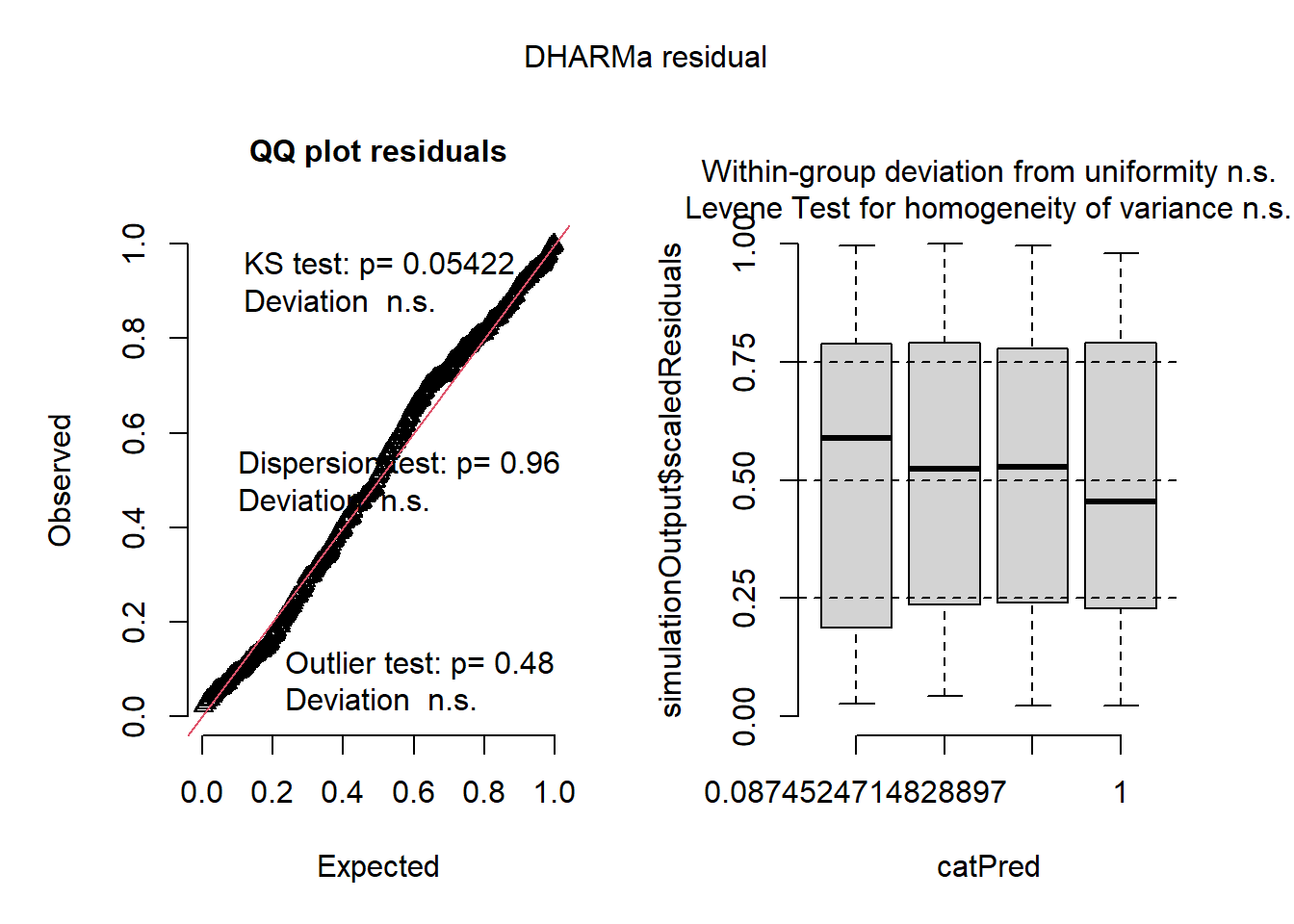
res_tmb2  <- simulateResiduals(owls_tmb_nb2, plot = FALSE)
plot(res_tmb2)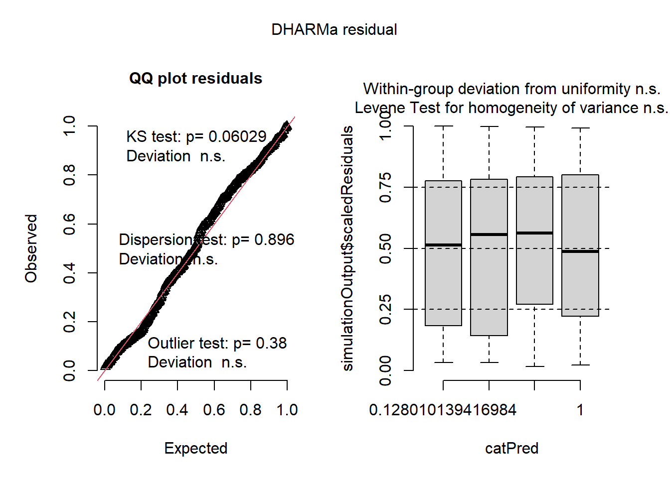
Based on these plots, both “glmmTMB” models also fit!
QQ Plot
- residuals are uniform
- negative binomial family captures variance structure
- no problematic outliers
Residuals by Predicted Bins
- shows no heteroscedasticity and no systematic pattern in residuals vs fitted values
- no bias at low or high predicted values
Let’s evaluate performance again
tidy(owls_tmb_nb1, effects = "fixed", conf.int = TRUE)## # A tibble: 4 × 9
## effect component term estimate std.error statistic p.value conf.low
## <chr> <chr> <chr> <dbl> <dbl> <dbl> <dbl> <dbl>
## 1 fixed cond (Intercept) 2.25 0.0753 29.9 9.56e-197 2.11
## 2 fixed cond FoodTreatmen… -0.226 0.112 -2.02 4.29e- 2 -0.445
## 3 fixed cond SexParentMale -0.0184 0.0859 -0.215 8.30e- 1 -0.187
## 4 fixed cond FoodTreatmen… 0.0347 0.137 0.253 8.00e- 1 -0.234
## # ℹ 1 more variable: conf.high <dbl>tidy(owls_tmb_nb2, effects = "fixed", conf.int = TRUE)## # A tibble: 4 × 9
## effect component term estimate std.error statistic p.value conf.low
## <chr> <chr> <chr> <dbl> <dbl> <dbl> <dbl> <dbl>
## 1 fixed cond (Intercept) 2.23 0.0809 27.6 6.74e-168 2.07
## 2 fixed cond FoodTreatmen… -0.181 0.117 -1.55 1.21e- 1 -0.409
## 3 fixed cond SexParentMale -0.0122 0.0924 -0.132 8.95e- 1 -0.193
## 4 fixed cond FoodTreatmen… 0.00957 0.143 0.0667 9.47e- 1 -0.272
## # ℹ 1 more variable: conf.high <dbl>Based on this model, there is still no strong evidence that either food treatment or parent sex meaningfully changes the rate of begging calls. The results of the “glmmTMB” model are identical in direction and magnitude to the “lme4” model. We see the same results with the \(R^2\) values below:
r2_nakagawa(owls_tmb_nb1)## # R2 for Mixed Models
##
## Conditional R2: 0.094
## Marginal R2: 0.025r2_nakagawa(owls_tmb_nb2)## # R2 for Mixed Models
##
## Conditional R2: 0.100
## Marginal R2: 0.017So if both our models fit well and have similar results, how can we test which one is actually the best?
Start by comparing the AIC
AIC(owls_lme4_nb, owls_tmb_nb1, owls_tmb_nb2)## df AIC
## owls_lme4_nb 6 2763.182
## owls_tmb_nb1 6 2760.309
## owls_tmb_nb2 6 2763.023Compare our \(R^2\) values
r2_nakagawa(owls_lme4_nb)## # R2 for Mixed Models
##
## Conditional R2: 0.099
## Marginal R2: 0.017r2_nakagawa(owls_tmb_nb1)## # R2 for Mixed Models
##
## Conditional R2: 0.094
## Marginal R2: 0.025r2_nakagawa(owls_tmb_nb2)## # R2 for Mixed Models
##
## Conditional R2: 0.100
## Marginal R2: 0.017We can also compare log-likelihood
logLik(owls_lme4_nb)## 'log Lik.' -1375.591 (df=6)logLik(owls_tmb_nb1)## 'log Lik.' -1374.155 (df=6)logLik(owls_tmb_nb2)## 'log Lik.' -1375.512 (df=6)We can go back and compare the diagnostics plots but I think we can safely call this a tie between models! (Maybe a slight victory for owls_tmb_nb1)
However, there are some instances where this may not be the case. Here is a general overview of the difference between the two packages:
lme4 is better when…
- You want simplicity and transparency.
- You have standard response families (e.g., Gaussian, Binomial, Poisson…)
- You don’t need zero-inflation or complex variance structures.
- Your model is small/medium-sized and converges easily.
glmmTMB shines when…
- Your data are zero-inflated or truncated.
- You need flexible distributions.
- You need to model the dispersion itself (heterogeneous variance).
- You’re doing model selection or prediction at scale.
- You need complex random structures or correlated random effects.
Lets try the glmmTMB() function with our full dataset from earlier (zero-inflated)
# Baseline NB (no ZI factor)
m_nb <- glmmTMB(SiblingNegotiation ~ FoodTreatment * SexParent + (1|Nest),
data = Owls, family = nbinom2())

# Zero-inflated NB: a ZI component (~ 1) adds extra zeros
m_zinb <- glmmTMB(SiblingNegotiation ~ FoodTreatment * SexParent + (1|Nest),
ziformula = ~ 1,
data = Owls, family = nbinom2())

# Hurdle NB: zero vs positive modeled separately
m_hurd <- glmmTMB(SiblingNegotiation ~ FoodTreatment * SexParent + (1|Nest),
ziformula = ~ 1,              # hurdle uses 'truncated_nbinom2' for count
data = Owls,
family = truncated_nbinom2())
Now we can compare the glmmTMB() models
AIC(m_nb, m_zinb, m_hurd)## df AIC
## m_nb 6 3499.763
## m_zinb 7 3425.483
## m_hurd 7 3432.816The glmmTMB() model with the zero inflation factor performed the best based on AIC. For your exercise you will use all evaluation criteria but we will skip that for now.
Here is how you can interpret a zero-inflated model
- Conditional model (count part): effects on mean calls when calling is possible.
- ZI model (zero part): effects on the odds of structural zero.
summary(m_zinb)$coefficients## $cond
## Estimate Std. Error z value
## (Intercept) 2.22379780 0.09261448 24.0113406
## FoodTreatmentSatiated -0.31423249 0.13758345 -2.2839410
## SexParentMale -0.02595704 0.10247113 -0.2533108
## FoodTreatmentSatiated:SexParentMale 0.06321679 0.16152295 0.3913796
## Pr(>|z|)
## (Intercept) 2.117048e-127
## FoodTreatmentSatiated 2.237500e-02
## SexParentMale 8.000281e-01
## FoodTreatmentSatiated:SexParentMale 6.955167e-01
##
## $zi
## Estimate Std. Error z value Pr(>|z|)
## (Intercept) -1.209909 0.1128472 -10.72166 8.054478e-27
##
## $disp
## NULLEffect Display
library(effects)## Loading required package: carData## lattice theme set by effectsTheme()
## See ?effectsTheme for details.pred_zinb <- allEffects(m_zinb)## Warning in Effect.glmmTMB(predictors, mod, vcov. = vcov., ...): overriding
## variance function for effects/dev.resids: computed variances may be incorrectplot(pred_zinb, main = "ZI-NB model effects")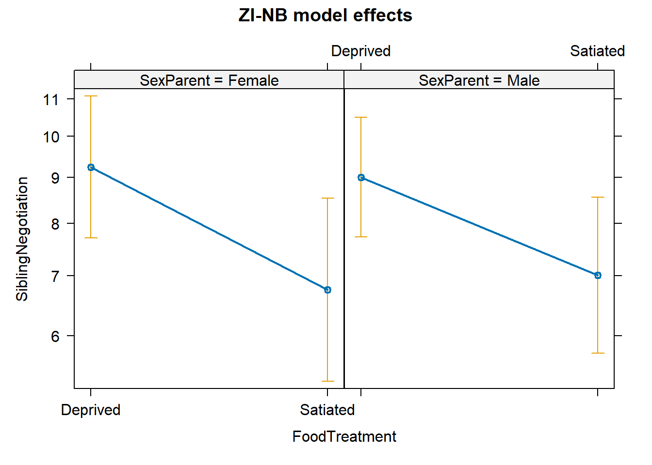
The plot shows how the predictors influence the expected counts when calling actually happens (non-zero).
Now that we’ve gone through the differences between lme4() and glmmTMB() as well as how to include zero inflation… its your turn!
Your goal: decide which model best explains begging calls in the full dataset and justify it with diagnostics.
- Get the full Owls dataset.
- Select your predictors (they should be different than the ones in the example).
- Build three models with the Owls data:
- NB GLMM with lme4()
- NB GLMM with glmmTMB()
- ZI-NB with glmmTMB()
- Choose three types of model comparison (e.g. AIC, visual assessment of diagnostics, \(R^2\), etc.) to determine which model is best.
- Create a prediction figure from your chosen model.
- Describe your model results in ecological context (a few sentences).