Lab 1: Algorithms in R
NRES 746
Fall 2025
In this course we use the R programming language for statistical computing and graphics, The purpose of this laboratory exercise is to develop familiarity with programming in R.
Lab 1 logistics
This lab provides an introduction to the R programming Language and the use of R to perform statistical and programming tasks. As with all lab reports, your answers will either take the form of R functions or short written responses. The R functions should be stored in an R script file (‘.R’ extension). To allow me to evaluate your work more efficiently, please name your R script using the following convention: “[your first name]_[your last name]_lab1.R”. So my submission would be “kevin_shoemaker_lab1.R” (all lower case).
Please include only the requested functions in your submitted R script. That is, the R script you turn in should only include the custom R functions you constructed to answer the questions, and none of the ancillary code you used to develop and test your functions. You will probably want to complete the lab exercises using a ‘full working version’ of your script (that includes all your work, including code for testing your solutions), and then save a reduced copy (containing only the requested functions and nothing more) for submission. Ask your instructor if you’d like a demonstration of how this works!
Before submitting your code using WebCampus, please clear your environment and run the script you will submit (containing only the requested functions) from start to finish. Check the ‘Environment’ tab in RStudio after running your script, and make sure that the script ONLY defines functions within your global environment- no other objects (data, values, etc.). The script you submit should generate no additional objects (e.g., data frames), it should not read in any files. Don’t put a ‘clear workspace’ line (e.g., ‘rm(list=ls()))’ anywhere in your submitted code- unless you want to make life difficult for the instructor…
Submit your R script (functions only) using WebCampus. Follow the above instructions carefully!
Submit short-answer responses using WebCampus. In addition to submitting your script, you will need to respond to additional questions using the Lab 1 “quiz” interface on WebCampus.
Please submit your R script and complete the WebCampus quiz by midnight on the due date (one week after the final lab session allocated for this topic). You can work in groups but submit the materials individually. Refer to WebCampus for due dates.
This lab exercise (Lab 1) will extend over two laboratory periods.
Getting started with R
- Go to website http://cran.r-project.org/. This is the source for downloading the free, public-domain R software and where you can access R packages, find help, access the user community, etc. If you haven’t already installed R, do so now!
- Open the Rstudio software (https://www.rstudio.com– and install if you haven’t done so already. Change the working directory to a convenient directory (e.g., a subfolder called ‘Lab 1’ in your main course directory). NOTE- if you set up an Rstudio “project” (.Rproj extension) in this directory, the working directory is set automatically each time you load the project! I recommend you set up an R studio project for this course.
- Open a new, blank R script window in Rstudio. Using comments (anything preceded by a hash mark is not interpreted by R and can be used to provide human-readable notes and commentary so your code is more readable), add a header to the script to indicate that this is lab 1- include your name and the course number in the header.
- Save the script to your working directory. You will be submitting a reduced version of this script (requested functions only) via NevadaBox when you have finished all the exercises.
- While you’re at it, I recommend starting a new Word document or Google Doc to record your written responses to the lab exercises. When you’re ready, you can copy and paste your responses from this document directly into WebCampus (rather than writing your responses into webcampus directly).
Take some time to get more familiar with R!
This is the only lab period we will devote to learning R- after this we will assume you have proficiency with defining variables and functions, reading in datasets, visualizing data, etc. in R.
From the R manual, ‘Introduction to R’ you can implement all the steps in Appendix A, located here. This takes you far but without much explanation– it is a way to jump into the deep end of the pool.
Alternatively, or in addition, go to the Links page and pick a tutorial to run through (e.g., the Datacamp introductory R course, which uses the ‘tidyverse’ packages). You can also check out the materials from my R “bootcamp” archive.
Before you move on, make sure you have a basic understanding of how to work with R and RStudio. If you are working with someone who has used R before, don’t be afraid to ask questions! Take your time with this- you might want to use the entire lab period on this if you have never used R before - it will be time well spent!
Another useful introductory R tutorial can be found here, courtesy of NCEAS. If you haven’t used R before, consider working through this tutorial before going through the lab exercises.
If you already have basic R expertise, you can move ahead!
Some Preliminary Practice with R
Here we will get warmed up for the lab exercises.
Part 1- define a function
Write a function that takes a numeric input vector and computes the sum of all its elements.
Basically, all you need to do here is write ‘sum(x)’ where it says ‘[add code here]’
NOTE: you don’t need to submit this as part of your lab report! This is just practice…
 # demo function (not part of lab)

myfunc <- function(x){
    # [add code here!]
}
Part 2: Central Limit Theorem (CLT)
To gain some familiarity with using R scripts and developing algorithms, complete the following exercise (you don’t need to submit this demo as part of your lab write-up BUT you will be asked to use this code as part of exercise 1 (below).
Complete the following steps:
Review the meaning of the Central Limit Theorem, which states that the sum (or mean) of a sufficiently large number of independent and identically distributed random variables will form another random variable that is asymptotically normally distributed (as the number of elements added together approaches infinity), regardless of the distribution of the underlying data. One of the key implications is that the sample mean (sum of iid random variables divided by the sample size) will be normally distributed with mean equal to the mean of the data distribution and variance equal to the variance of the data distribution divided by the sample size:
\[X \sim any \;distribution(mean=\mu, var=\sigma^2)\]
Note that, although the normal distribution is the only distribution that is fully determined by its mean and variance, all probability distributions have a mean and variance (although some distributions ‘misbehave’ and have infinite mean and/or variance!).
\[ \bar{X}= \frac{1}{N}\sum_{i=1}^N X_i\] \[\bar{X} \xrightarrow{D} Normal(\mu,\frac{\sigma}{\sqrt{N}})\]
Type (or paste) the following code into your R script window (or RStudio script window):
# CENTRAL LIMIT THEOREM demonstration ------------------------

N <- 10          # sample size
lots <- 1000       # placeholder representing infinity

##  Define the random number distribution. ------------------

runif(N,10,20)   # try uniform random number generator with min of 10 and max of 20.
## [1] 14.91297 12.51504 15.80130 14.46472 19.01532 11.30745 16.55575 13.83633
## [9] 19.29822 15.12409many_samples = replicate(lots,runif(N,10,20)) # do it many times!
many_xbars = colMeans(many_samples)
hist(many_samples,freq=F,ylim=c(0,1),main="",xlab="Value") # plot out the distribution of sample means
hist(many_xbars,freq=F,add=T,col="red") # overlay the distribution of the underlying data from which we are drawing samples.
legend("topleft",fill=c("gray","red"),legend=c("data population","sample means"),bty="n") # add a legend to the plot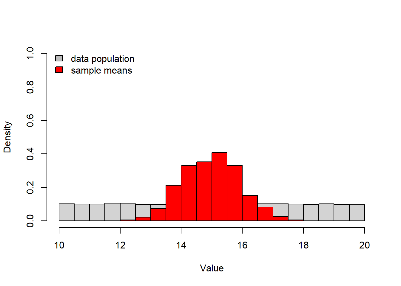
- Experiment with executing this code in the following four ways:
- copy and paste from the script window directly into the R
console
- use
to execute line by line from within the script window in RStudio; (or on Macs, use command enter)
- use
to select the whole code block, then to execute all at once - highlight any block of code and run only that block using
- save the script to your working directory as a text file with .R extension, open a new script and then run the script from the new script using the “source()” function, e.g.:
- copy and paste from the script window directly into the R
console
source("CentralLimitTheorem.R") # run the R script from a different script!
NOTE: The hash (#) used in the above code allows you to insert comments adjacent to snippets of code, which facilitates readability of code (and lets the programmer remember later on what he/she was thinking when coding things a certain way!). It is good practice to comment every line of code so as to describe what it does in plain English, including all variables and functions. Make sure you fully understand the commented code for the CLT demonstration above!
- Now modify your R script to see how closely the distribution of sample means follows a normal distribution. Use a “quantile-quantile” (q-q) plot to visualize how closely the quantiles of the sampling distribution resemble the quantiles of a normal distribution. Use the “qqnorm()” function. To learn more about this function, type:
?qqnorm # learn more about the "qqnorm()" functionPlot the q-q plot next to the histograms. The plot on the left should be the comparison of histograms (for population distribution and distribution of sample means) shown in the original script (above). The plot on the right should be the q-q plot. To produce side-by-side plots, you will need to add this line of code to the appropriate place in your script:
# Set graphical parameters for side by side plotting -------------

par(mfrow=c(1,2)) # sets up two side by side plots as one row and two columns

## or alternatively...

layout(matrix(1:2,nrow=1))
In addition, run a Shapiro-Wilk normality test, which tests the null hypothesis that a set of numbers (in this case the vector of sample means) indeed comes from a normal distribution (so what does a low p-value mean??). Use the “shapiro.test()” function:
?shapiro.testSo… what can you conclude from these tests??
Exercise 1: custom functions!
Finally we have arrived at the ACTUAL lab exercises. Remember you don’t need to submit any of the work up to this point.
For the first part of this lab, you are asked to write several functions (and submit them as part of your lab script, of course!). The functions increase quickly in complexity!
You should now know how to construct functions in R. If you don’t, go back to the NCEAS tutorial and review the section on writing functions.
Exercise 1a (code)
Write an R function called “CoefVar()” that takes a numeric vector (named ‘x’ within the function but could have any name outside the function) as input, and computes (and returns) its coefficient of variation (CV; standard deviation as a proportion of the mean). To make sure it works, apply your function to the ‘Height’ vector in the ‘trees’ dataset that installs with R as sample data:
You can use the following code to test your function using the built-in ‘trees’ dataset.
# Testing your code ------------------------
#   Explore the "trees" dataset

#?trees

summary(trees)    # learn more about the data
## Girth Height Volume
## Min. : 8.30 Min. :63 Min. :10.20
## 1st Qu.:11.05 1st Qu.:72 1st Qu.:19.40
## Median :12.90 Median :76 Median :24.20
## Mean :13.25 Mean :76 Mean :30.17
## 3rd Qu.:15.25 3rd Qu.:80 3rd Qu.:37.30
## Max. :20.60 Max. :87 Max. :77.00trees$Height # extract the "Height" column from the trees dataset.## [1] 70 65 63 72 81 83 66 75 80 75 79 76 76 69 75 74 85 86 71 64 78 80 74 72 77
## [26] 81 82 80 80 80 87CoefVar(trees$Height) # run your new function!## [1] 0.08383964Exercise 1b (code)
Write a function called “DrawLine()” for drawing a regression line through a scatter plot. This function should be specified as follows:
- input:
- x = a numeric vector specifying the x-coordinates of the scatter
plot
- y = a numeric vector specifying the y-coordinates of the scatter plot
- x = a numeric vector specifying the x-coordinates of the scatter
plot
- suggested algorithm (base R):
- with the x and y coordinates, first produce a scatterplot (HINT: use the “plot()” function)
- use the “lm()” function to regress the y variable on the x variable.
- record the intercept and slope of the linear relationship between x and y (HINT: use the “coef()” function)
- add a regression line to the scatter plot (HINT: use the “abline()” function)
- suggested algorithm (ggplot):
- use the “lm()” function to regress the y variable on the x variable, and store the coefs
- make a data frame containing the x and y coordinates
- use ggplot to produce a scatterplot (HINT: use geom_point)
- add a regression line to the scatter plot (HINT: use the “geom_smooth” function with method “lm”)
- NOTE: you need to use the ‘print’ function to make sure your plot shows up when you run the function (e.g., ‘print(myplot)’)
- return:
- coefs = a vector of length 2, storing the intercept and slope of the linear relationship (in that order)
As a test, apply this function to the ‘Height’ (x axis) and ‘Volume’ (yaxis) vectors in the ‘trees’ dataset, and then to the ‘waiting’ (x axis) and ‘eruptions’ (y axis) vectors in the ‘faithful’ dataset.
#DrawLine(trees$Height,trees$Volume)

# ?faithful
# summary(faithful)

## ggplot version:
DrawLine(faithful$waiting,faithful$eruptions)    # test your function using the old faithful eruptions data
## `geom_smooth()` using formula = 'y ~ x'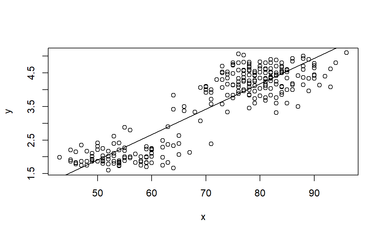
## (Intercept)           x
## -1.87401599  0.07562795
## base R version:
DrawLine_base(faithful$waiting,faithful$eruptions)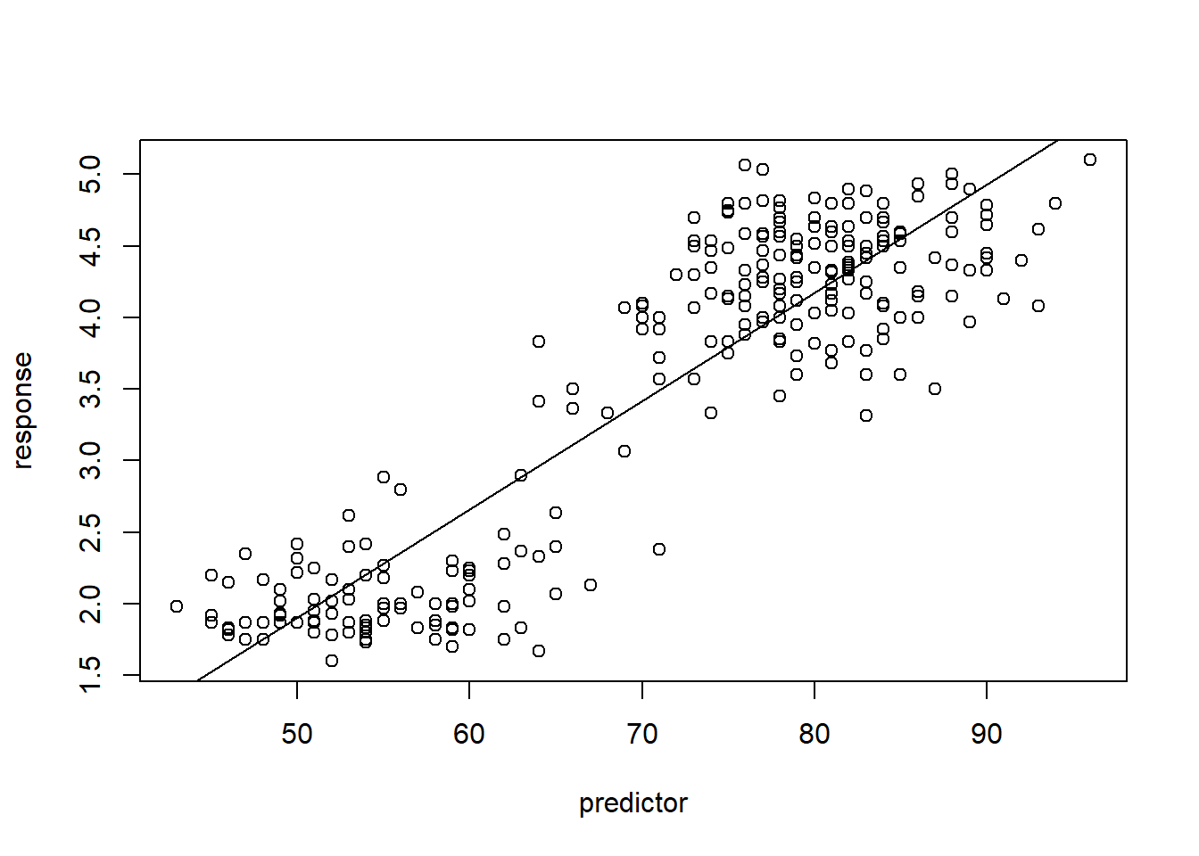
## (Intercept)           x
## -1.87401599  0.07562795
Exercise 1c (code)
Write a function called “DrawLine2()” for drawing a “smoothed” regression line through a scatter plot, making the smoothing span (degree of smoothness, or non-wiggliness of the line) a user-defined option. This function should be specified as follows:
- input:
- x = a numeric vector specifying the x-coordinates of the scatter
plot
- y = a numeric vector specifying the y-coordinates of the scatter plot
- smooth = a logical (TRUE/FALSE) value defining whether or not to add a smoothed line or a linear regression line
- span = a number indicating the degree of smoothness, or “un-wiggliness” of the smoothed line (only applies if smooth=TRUE)
- x = a numeric vector specifying the x-coordinates of the scatter
plot
- suggested algorithm (base R):
- with the x and y coordinates, first produce a scatterplot (HINT: use the “plot()” function)
- if smooth is FALSE, then proceed to draw a straight line as before (and return the coefficients)
- if smooth is TRUE, plot a smoothed, locally-weighted regression of the y variable on the x variable (e.g., using the “scatter.smooth()” function). Make sure you use the “span” argument!
- if smooth is TRUE, use the “loess()” function to record the same smoothed, locally-weighted regression of the y variable on the x variable. Again, make sure you use the “span” argument!
- suggested algorithm (ggplot):
- if smooth=TRUE, use the “loess()” function to regress the y variable on the x variable, and store the coefs. Otherwise store the ‘lm’ coefficients as before.
- make a data frame containing the x and y coordinates
- use ggplot to produce a scatterplot (HINT: use ‘geom_point’)
- add a regression line to the scatter plot (HINT: use the “geom_smooth” function with method “lm”). If smooth is TRUE, use the ‘loess’ method with specified span, otherwise use ‘lm’.
- NOTE: you need to use the ‘print’ function to make sure your plot shows up when you run the function (e.g., ‘print(myplot)’)
- return:
- out = (if smooth=TRUE) the loess model (the output produced by running “loess()” (or the slope and intercept from the linear regression, if smooth=FALSE)
Try testing your function using the trees and faithful datasets!
xvec <- c(1:10)
yvec <- rnorm(length(xvec),c(2:6,7:3),2)
DrawLine2(xvec,yvec,smooth=T,span=1)    # run your new function!
## `geom_smooth()` using formula = 'y ~ x'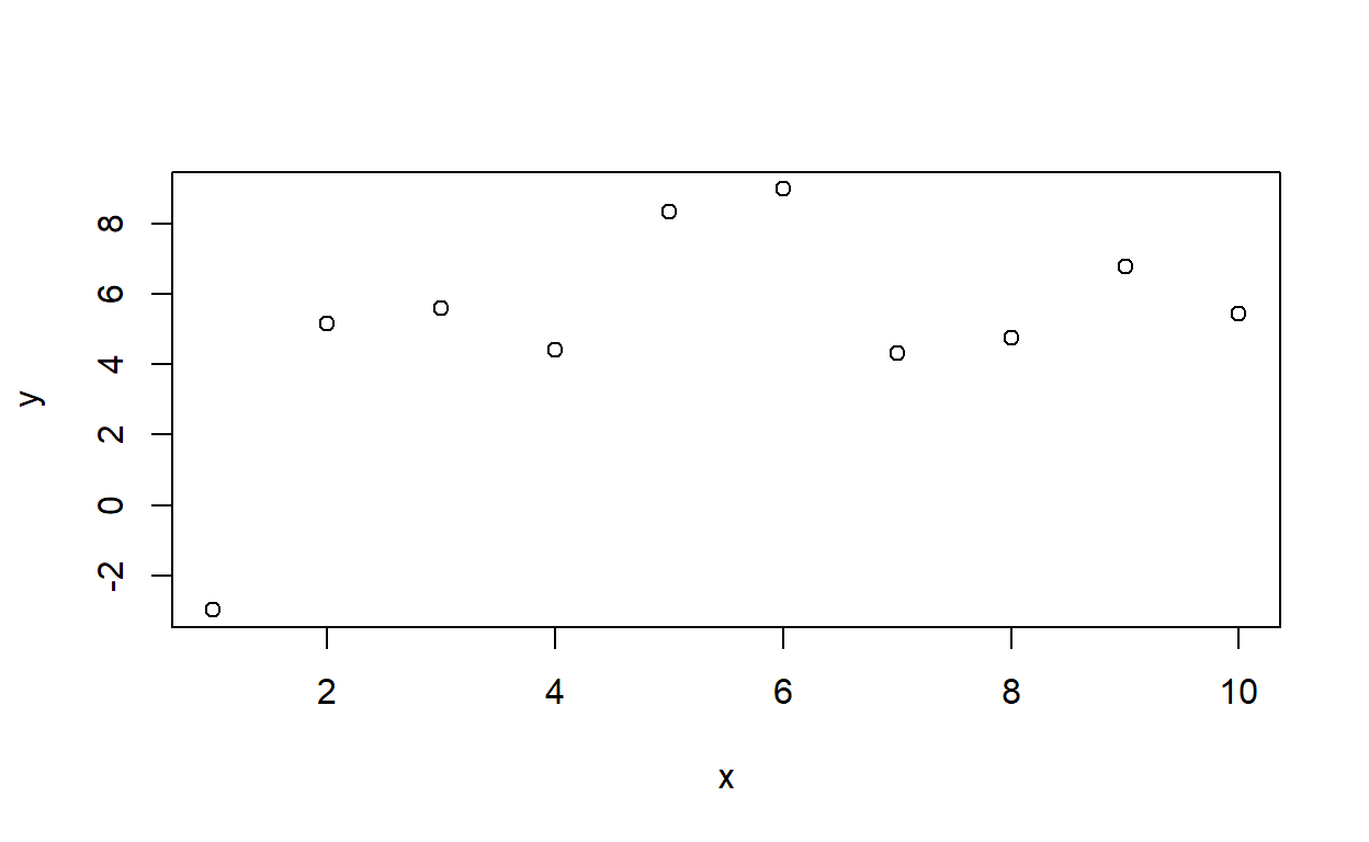
## Call:
## loess(formula = y ~ x, span = span)
##
## Number of Observations: 10
## Equivalent Number of Parameters: 3.45
## Residual Standard Error: 1.634DrawLine2(x=trees$Height,y=trees$Volume,smooth=F)## `geom_smooth()` using formula = 'y ~ x'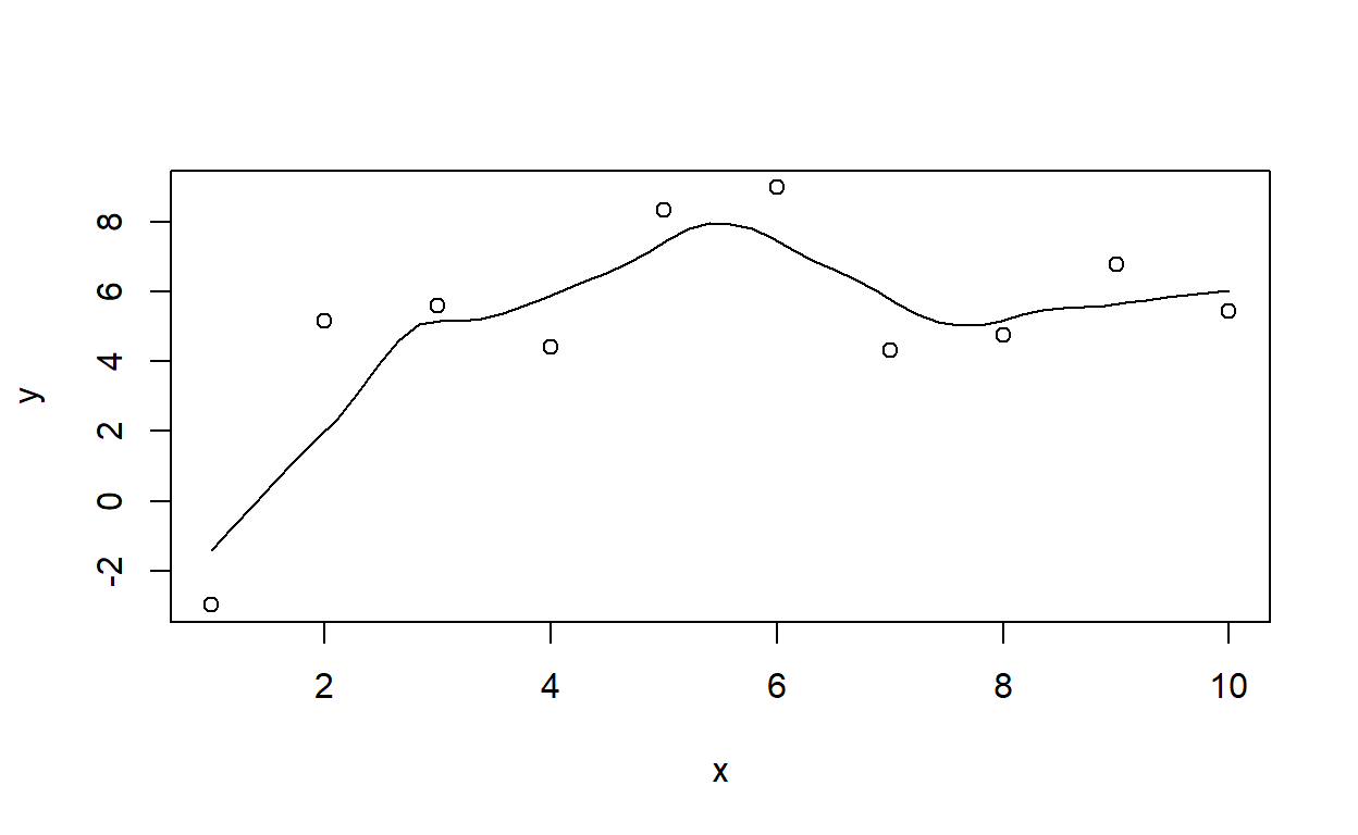
## (Intercept)           x
##   -87.12361     1.54335
DrawLine2(faithful$waiting,faithful$eruptions,smooth=T,span=1) # test using the old faithful eruptions data## `geom_smooth()` using formula = 'y ~ x'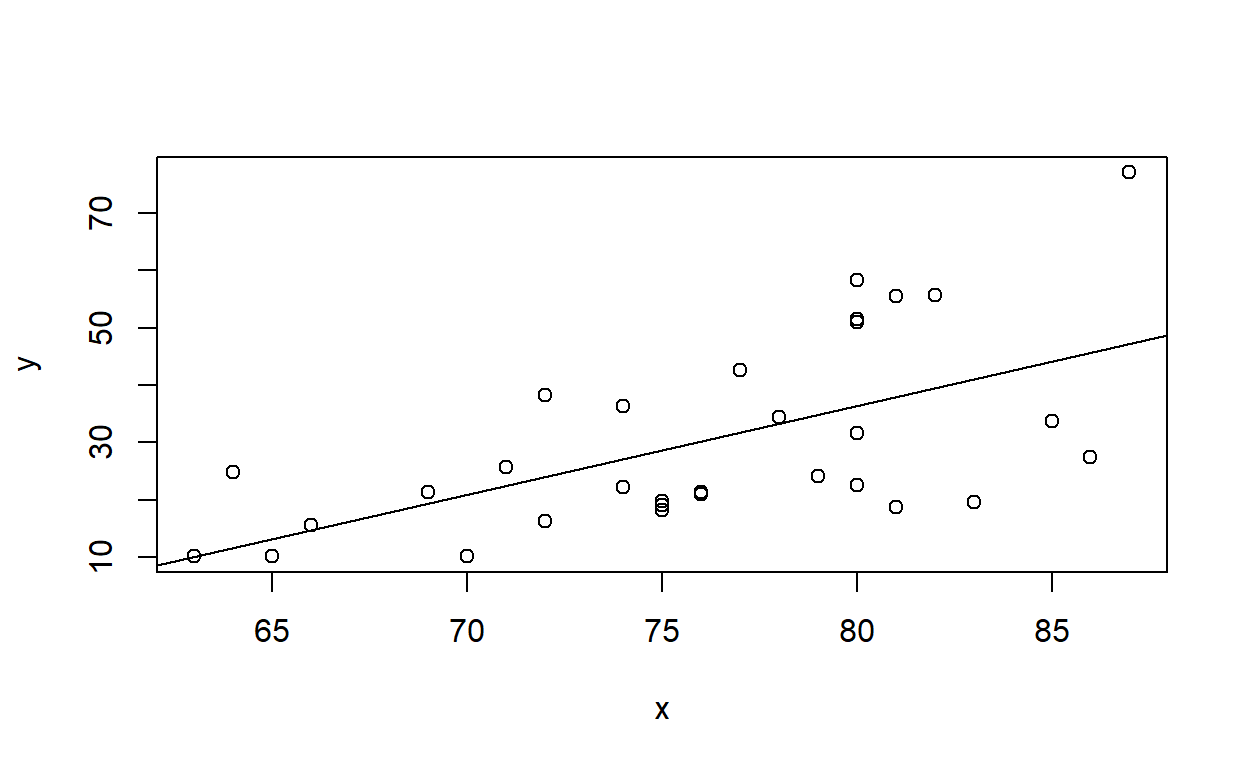
## Call:
## loess(formula = y ~ x, span = span)
##
## Number of Observations: 272
## Equivalent Number of Parameters: 3.4
## Residual Standard Error: 0.4274DrawLine2(faithful$waiting,faithful$eruptions,smooth=T,span=1.9)## `geom_smooth()` using formula = 'y ~ x'
## Call:
## loess(formula = y ~ x, span = span)
##
## Number of Observations: 272
## Equivalent Number of Parameters: 3.08
## Residual Standard Error: 0.4639
Exercise 1d (code)
Write a function called “CLTdemo()” based on the central limit theorem (CLT) demonstration code above. This function should be specified as follows:
- input:
- N = sample size (size of random sample) (default = 10)
- min = lower bound of the uniform distribution to draw from (default=0)
- max = upper bound of the uniform distribution (default=1)
- visualize = logical indicator of whether or not to produce visual tests for normality
- suggested algorithm:
- see CLT demonstration above! Note that you shouldn’t generate more than 5000 sample means- this is because the shapiro-wilks test only works for vectors less than or equal to 5000 in length.
- if visualize=TRUE, generate side-by-side plots of the histogram of sample means (left) and a quantile-quantile plot for visual tests of normality.
- return:
- out = the p-value from a Shapiro-Wilks normality test (the output produced by running “shapiro.test()” on the sample means)
And you can test your code with the following command:
CLTdemo(3,10,20) # run your new function!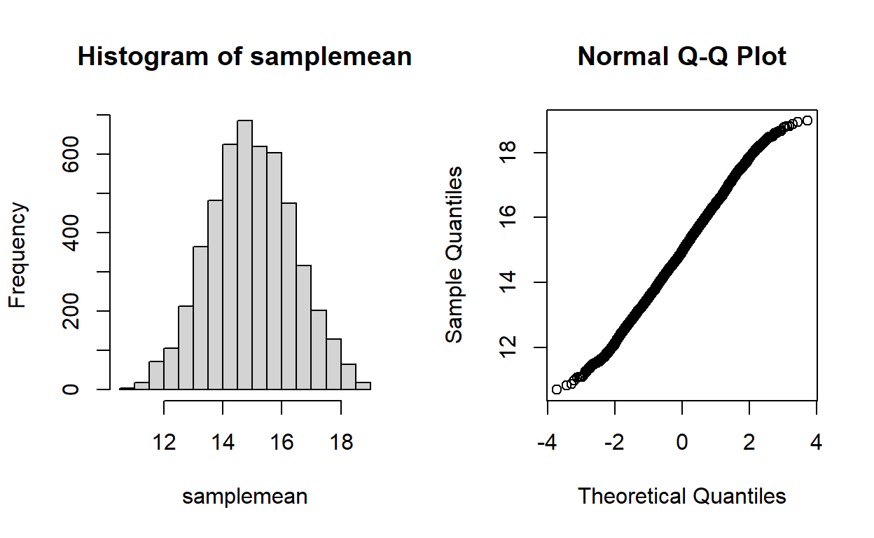
## [1] 0.006422794 ## you might want to replicate this many times...
replicate(5,CLTdemo(3,10,20,visualize=F)) # for example, replicate 5 times## [1] 0.02666252 0.22219402 0.14816431 0.04354325 0.01335300Exercise 1e (written response)
Finally, test the CLT function out for different parameter combinations to make sure it works! See if you can use this function to develop a reasonable rule for how large a sample size is necessary to ensure that the sample mean statistic (\(\bar{X}\)) is normally distributed given that the underlying data population is a uniform distribution.
Use your “CLTdemo” function to develop a rule for how large a sample size (N) is needed to ensure that the sample mean is normally distributed, given that the underlying data follows a uniform distribution. Please justify your answer!
Please submit your answer in WebCampus- and please justify your answer! [note: I am just looking for a thoughtful response, not a definitive mathematical proof! Just a few sentences is fine.]
Aside: default values in functions
NOTE: to set default values, just use the equals sign when defining your function. For example, say I wanted to write a function that adds the numbers in vector input ‘x’ OR adds a scalar input ‘y’ to each element of vector ‘x’. With only 1 input (‘x’) the function will sum up the elements in ‘x’. If the user specifies two arguments (x and y) then the function will add y to each element of x. It might look something like this:
newsum <- function(x,y=NULL){
  if(is.null(y)) sum(x) else x+y
}

newsum(5:10)   # use default value of y
## [1] 45newsum(5:10, 2) ## [1] 7 8 9 10 11 12Try setting some alternative default values and re-running the function with and without arguments until you are sure you understand how default values work!
Exercise 2: regression in R (written responses in WebCampus)
Before we start with the exercise, here is some background:
- Type the following for a list of sample datasets that come with the core R package (some of these you have already encountered).
library(help = "datasets")    # list of sample datasets that come with R
?airquality    # this is the dataset we'll work with in this exercise
Examine the ‘airquality’ dataset (use the ‘head’ and ‘summary’ functions). Note that there are missing values where ozone concentration data and solar radiation data were not collected.
We could ignore the missing values and just go ahead with our regression analysis, since the default response of the “lm()” (‘linear model’) function is to omit cases with missing values in any of the specified parameters. However, to avoid problems later, we will omit them explicitly by constructing a new, ‘cleaned’ dataset as follows:
air_cleaned <- na.omit(airquality) # remove rows with missing dataConduct a multiple linear regression of ozone concentration as a function of solar radiation, wind and temperature. Use the ‘lm()’ function to conduct an ordinary least squares (OLS) regression analysis.
Explore the regression outputs using the ‘summary’ function, and explore regression diagnostics:
par(mfrow=c(3,2))
plot(model1, which=c(1:4))   # diagnostic plots (NOTE: the 'plot()' function returns these plots by default when the input is a linear regression model)


hist(residuals(model1), breaks=10)   # histogram of residuals
plot(predict(model1) ~ air_cleaned$Ozone)     # plot predicted vs observed- should follow 1:1 line. Examine this for model biases.
abline(0,1)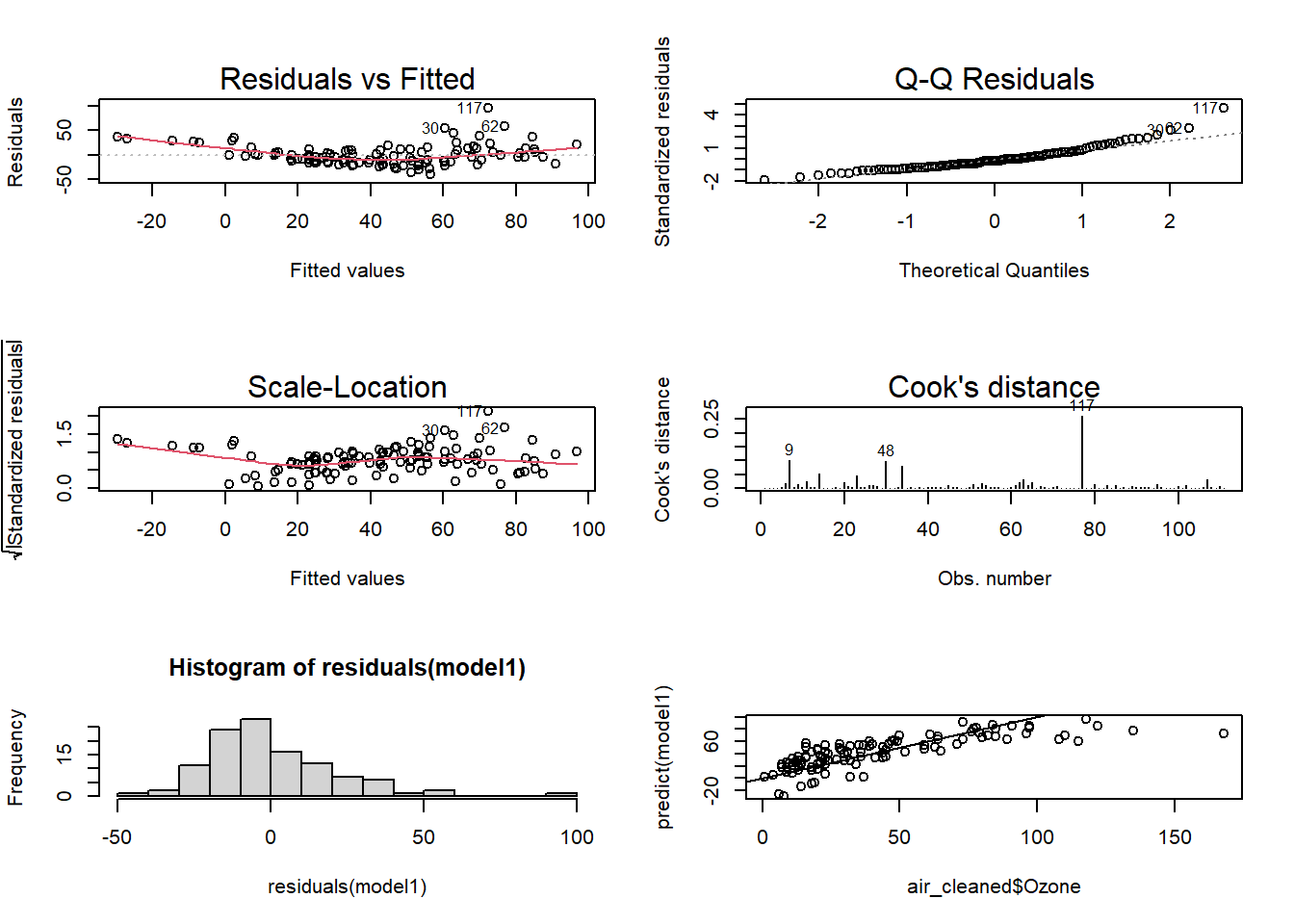
NOTE: see this website for more information on the diagnostic plots produced by lm().
- Consider the possibility that there may be an important interaction effect between solar radiation and temperature on influencing ozone concentrations. Explore that with a scatter plot where symbol size is scaled to ozone concentration:
coplot(air_cleaned$Ozone~air_cleaned$Temp|air_cleaned$Solar.R,rows=1) # the "|" operator can be read "conditional on"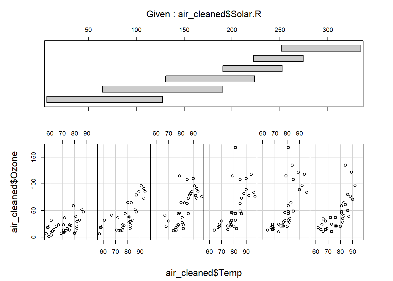
       # alternatively, you can use ggplot
library(ggplot2)
ggplot(air_cleaned,aes(Temp,Solar.R)) +
  geom_point(aes(size=Ozone))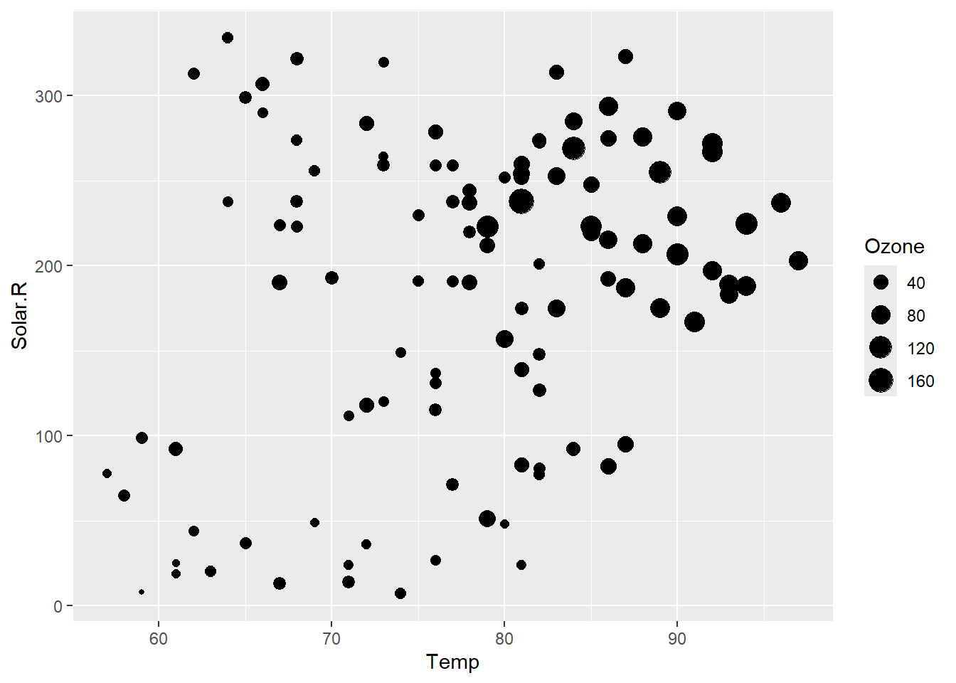
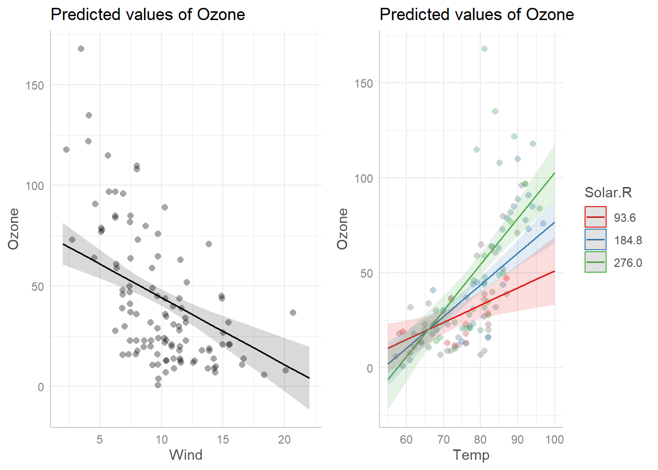
- Now fit a second model that includes the interaction between solar radiation and temperature. Use the following formula to fit the interaction:
formula2 <- "Ozone ~ Wind + Solar.R * Temp" # you can name formulas...Explore regression diagnostics and coefficients for the second model in the same way as you did for the first model without the interaction term.
Conduct a test to formally test whether the more complex model (including the interaction term) fits the data significantly better than the reduced model (with fewer parameters) that lacks the interaction term. Recall that the \(R^2\) value is inadequate for this purpose because \(R^2\) will always increase with additional parameters! Use the following syntax,
anova(model1, model2, test="Chisq") Very briefly (but in complete sentences) answer the following questions in WebCampus:
Exercise 2a (written response)
By how much (and in what direction) is ozone concentration expected to change if temperature increased from 26 to 30 degrees Celsius? Assume that solar radiation stays constant at 200 lang and wind speed stays constant at 9 mph. Be careful with the units for temperature! Make sure to use the ‘interaction’ model (model2) from part 7 above to answer this question. Please briefly explain (in WebCampus) how you got your answer.
Exercise 2b (written response)
Briefly, what is the null hypothesis that the p-values for the individual regression coefficients are designed to test?
Exercise 2c (written)
Based on your diagnostic plots, do you think this is an appropriate model for these data? Explain your reasoning.
Exercise 2d (written)
Which of the predictor variables you included in your model is the most important in predicting ozone concentration? Explain your reasoning.
## Analysis of Variance Table
##
## Response: Ozone
##               Df Sum Sq Mean Sq F value    Pr(>F)
## Wind           1  45694   45694 112.708 < 2.2e-16 ***
## Solar.R        1   9055    9055  22.335 7.072e-06 ***
## Temp           1  19050   19050  46.988 4.901e-10 ***
## Solar.R:Temp   1   5028    5028  12.402 0.0006337 ***
## Residuals    106  42975     405
## ---
## Signif. codes:  0 '***' 0.001 '**' 0.01 '*' 0.05 '.' 0.1 ' ' 1
## Single term deletions
##
## Model:
## Ozone ~ Wind + Solar.R * Temp
## Df Sum of Sq RSS AIC Pr(>Chi)
## <none> 42975 671.43
## Wind 1 11679.6 54654 696.12 2.393e-07 ***
## Solar.R:Temp 1 5028.2 48003 681.71 0.0004573 ***
## ---
## Signif. codes: 0 '***' 0.001 '**' 0.01 '*' 0.05 '.' 0.1 ' ' 1##
## Call:
## lm(formula = Ozone ~ scale(Wind) + scale(Solar.R) * scale(Temp),
## data = air_cleaned)
##
## Residuals:
## Min 1Q Median 3Q Max
## -39.634 -12.505 -2.300 8.956 94.162
##
## Coefficients:
## Estimate Std. Error t value Pr(>|t|)
## (Intercept) 39.996 2.002 19.976 < 2e-16 ***
## scale(Wind) -11.879 2.213 -5.367 4.74e-07 ***
## scale(Solar.R) 9.006 2.248 4.006 0.000115 ***
## scale(Temp) 15.844 2.297 6.898 3.98e-10 ***
## scale(Solar.R):scale(Temp) 7.216 2.049 3.522 0.000634 ***
## ---
## Signif. codes: 0 '***' 0.001 '**' 0.01 '*' 0.05 '.' 0.1 ' ' 1
##
## Residual standard error: 20.14 on 106 degrees of freedom
## Multiple R-squared: 0.6472, Adjusted R-squared: 0.6339
## F-statistic: 48.61 on 4 and 106 DF, p-value: < 2.2e-16Exercise 3: Algorithmic (brute force) z-test
Review the “brute-force z-test” code from the “Why focus on algorithms” lecture. Then complete the following exercises:
Exercise 3a (code)
What if we wanted to run a two-tailed z-test? That is, what if our alternative hypothesis were that salmon fed on the new vegetarian diet could plausibly be larger or smaller than those fed on the conventional diet after one year?
Modify the function (“ztest_bruteforce()”) with a new argument that allows for both one and two-tailed tests! Name your new function “my_ztest()”.
To convince yourself that your new function works, try running your function for a (made-up) case where the observed body mass for those fed on the new diet are generally higher than the expected body mass for those fed on the conventional diet after one year – the opposite of your hypothesis!
NOTE: you may get tangled up with the null hypothesis/p-value concept, which is admittedly a difficult concept! A p-value always assumes the null hypothesis is true (what is the probability that a random sample under the null hypothesis could give as much evidence for your alternative hypothesis than the data you observed?).
- In the case of salmon example, our original alternative hypothesis (one-tailed: lower) is that the treatment mean (veg. diet) is less than the null mean (convenction diet).
- We could have specified a different one-tailed hypothesis: that the treatment mean should be greater than the null mean (one-tailed: higher)
- Under a 2-tailed hypothesis, the direction of the difference doesn’t matter- we just think that the treatment mean should be different than the null mean.
Include your function in your submitted r script!
This function should be specified as follows:
- input:
- d = a vector of observed sample values (data)
- mu = a scalar value representing the expected mean value under the
null hypothesis
- sigma = a scalar value representing the population standard
deviation under the null hypothesis
- alternative = a character string with one of three possible values: ‘l’ to indicate a one-tailed “less than” alternative hypothesis, ‘g’ to indicate a “greater than” alternative, and “b” to indicate a 2-tailed test (default should be ‘b’)
- suggested algorithm:
- See lecture for example ‘brute force z-test()’ function
- To implement the two-tailed test, you need to define what ‘extreme’
means in both directions. You might first define the absolute difference
between the population mean (mu) and the sample mean. Then define ‘more
extreme’ as any simulated sample mean that falls further away from the
population mean in either direction (larger or smaller than mu) than the
observed sample mean.
- Use an “if-else” or “case_when” statement to accommodate all three possible alternative hypotheses.
- return:
- to_return = a named list with three elements: “x_bar”, representing
the sample mean (scalar) “nulldist”, representing many samples from the
sampling distribution for x_bar under the null hypothesis (vector)
“p_value”, representing the p-value (scalar)
- to_return = a named list with three elements: “x_bar”, representing
the sample mean (scalar) “nulldist”, representing many samples from the
sampling distribution for x_bar under the null hypothesis (vector)
Test your function using some alternative sample data values. For example:
mu = 4     # testing code
sigma = 2
mysample = c(3.14,3.27,2.56,3.77,3.34,4.32,3.84,2.19,5.24,3.09)
test = my_ztest(mysample, mu, sigma,alternative = 'l' )
str(test)
## List of 3
## $ Xbar : num 3.48
## $ nulldist: num [1:10000] 4.84 3.72 5.25 3.43 4.23 ...
## $ p_value : num 0.207test$p_value## [1] 0.2072 # also try using the code from lecture to compare against a "real" z-test!Also try using the code from lecture to compare against a “real” z-test– for example:
mu = 4     # testing code
sigma = 2
mysample = c(3.14,3.27,2.56,3.77,3.34,4.32,3.84,2.19,5.24,3.09)

samplemean = mean(mysample)    # real z-test
stderr <- sigma/sqrt(length(mysample))  # population standard error
zstat = (samplemean-mu)/stderr
pnorm(zstat)
## [1] 0.203689test = my_ztest(mysample, mu, sigma,alternative = 'l' ) # compare your function with the real answer
test$p_value## [1] 0.204library(BSDA)## Loading required package: lattice##
## Attaching package: 'BSDA'## The following object is masked from 'package:datasets':
##
## Orangez.test(x=mysample,mu=mu, sigma.x=sigma,alternative = "less") # 'canned' z-test##
## One-sample z-Test
##
## data: mysample
## z = -0.82852, p-value = 0.2037
## alternative hypothesis: true mean is less than 4
## 95 percent confidence interval:
## NA 4.516297
## sample estimates:
## mean of x
## 3.476Exercise 3b: (code)
Non-parametric test of sample mean vs null
Now, what if we had access to a large set of independent samples under the null hypothesis AND that we would like to relax the assumption that the data follow a normal distribution under the null hypothesis?
In this exercise, you are asked to modify the brute-force z-test function so that you generate your sampling distribution by simply sampling from the known data set under the null hypothesis. To do this you can use the ‘sample()’ function in R. For this purpose you should sample from the null with replacement. Here is an example:
## Exercise 3b -------

nulldata=c(2.2,3.86,6.39,4.6,3.43,5.16,4.36,4.22,6.31,4.61,5.13,4.12,4.64,4.03,5.01,7.33,5.35,4.7,2.82,4.87,3.87,5.95,5.28,4.02,3.58,4.03,5.38,5.5,3.07,3.29,3.45,5.25,5.7,1.26,5.28,4.19,4.76,4.2,4.81,2.5)
sample(nulldata,10,replace=T)    # use the sample function to sample from a large vector with replacement
For this exercise, we will return to the original null hypothesis: that salmon raised on the new diet will be smaller (lower mass) than those raised on conventional diet after one year.
Include your function in your submitted r script!
This function should be named ‘x_vs_null()’ and should be specified as follows:
- input:
- x = a vector containing the observed sample
- nulldata = a vector of observations under the null hypothesis (empirical null distribution)
- suggested algorithm:
- Instead of sampling from a normal distribution to simulate samples under the null hypothesis, use the ‘sample’ function to sample directly from the null data distribution.
- return:
- to_return = a named list with three elements: “xbar”, representing the sample mean, “nulldist”, representing the sampling distribution for sample means under the null hypothesis, and “p_value”, representing the p-value of the test
Test your function using some alternative sample data vectors. For example:
nulldata=c(2.2,3.86,6.39,4.6,3.43,5.16,4.36,4.22,6.31,4.61,5.13,4.12,4.64,4.03,5.01,7.33,5.35,4.7,2.82,4.87,3.87,5.95,5.28,4.02,3.58,4.03,5.38,5.5,3.07,3.29,3.45,5.25,5.7,1.26,5.28,4.19,4.76,4.2,4.81,2.5)
mysample = c(3.14,3.27,2.56,3.77,3.34,4.32,3.84,2.19,5.24,3.09)
test = x_vs_null(mysample, nulldata )
test$p_value
## [1] 0.008Exercise 4: Bootstrapping
Review the bootstrapping code from the first lecture topic (to generate confidence intervals for arbitrary test statistics). Then complete the following exercise:
Exercise 4a (code)
Generate a new R function, called “RegressionCoefs()” that takes a data frame as the first input parameter and the name of the response variable as the second input parameter, and returns the regression coefficients (\(\beta\)) produced by regressing the response variable on each predictor variable one at a time (returning a vector of regression coefficients). You can use the “Rsquared()” function (from the lecture) as a reference!
More specifically, this function should be specified as follows:
- input:
- df = a data frame containing the response variable and one or more predictor variables. All columns that are not the response variable are assumed to be predictor variables
- responsevar = the name of the column that represents the response variable.
- suggested algorithm:
- Follow the R squared example from lecture. Store the regression coefficients instead of the R-squared values.
- return:
- coefs = a vector of the regression coefficients (slope terms) for all predictor variables. This should be a vector with one element (slope term) for each predictor variable. The number of elements in your vector should be one fewer than the number of columns in your dataset. If possible, try to make this a named vector- with the name of each predictor variable associated with its respective coefficient.
Include your function in your submitted r script!
You can test your function using the following code:
RegressionCoefs(trees,"Volume") # should return two regression coefficients## Girth Height
## 5.065856 1.543350Exercise 4b: (code)
Generate a new R function, called “BootCoefs()” that meets the following specifications:
- inputs:
- “df” = a data frame that includes the response variable and all
possible predictor variables
- “statfunc” = a function for generating summary statistics (in this
case, regression coefficients) from a data frame (which you already
developed in part 1 of this challenge problem)
- “n_samples” = the number of bootstrapped samples to generate
- “responsevar” = the name of the response variable
- “df” = a data frame that includes the response variable and all
possible predictor variables
- algorithm:
- with the data frame, use the “boot_sample()” function provided in
the lecture to generate summary statistics for multiple bootstrap
samples. You do not need to modify the ‘boot_sample()’ function for this
problem
- Then, generate confidence intervals for each variable as the 2.5%, 50% and 97.5% quantile of the summary statistic for each predictor variable.
- with the data frame, use the “boot_sample()” function provided in
the lecture to generate summary statistics for multiple bootstrap
samples. You do not need to modify the ‘boot_sample()’ function for this
problem
- return: a matrix (rows=predictor vars, cols=2.5%, 50%, and 97.5% quantiles). Try to give the rows and columns proper labels!
Include your function in your submitted r script!
You can test your function using the following code:
BootCoefs(df=trees,fun=RegressionCoefs,1000,responsevar="Volume")## Girth Height
## 2.5% 4.362612 0.7690758
## 50% 5.027451 1.5358234
## 97.5% 5.632498 2.3628580df <- mtcars[,c(1,3,4,6)]
responsevar="mpg"
BootCoefs(df,RegressionCoefs,1000,responsevar)## disp hp wt
## 2.5% -0.05132901 -0.10073301 -7.100329
## 50% -0.04119646 -0.06940640 -5.377683
## 97.5% -0.03146126 -0.04591232 -4.166714Exercise 4c: (written)
To test your new function(s), generate bootstrapped confidence intervals around the regression parameters for your tree biomass regression. Compare these bootstrapped confidence intervals with the standard confidence intervals given by R in the “lm()” function. Are there any important differences? Explain your answer in WebCampus.
———— End of Lab 1! ——————–