Lab 2: Data Generating Models
NRES 746
Fall 2025
Please complete all assignments by the due date listed in WebCampus. You can work in groups but please submit the materials individually.
When writing functions, it’s often easiest to start off by writing a script, and then when you have everything working properly, wrap the script into a function.
Don’t forget to test your functions!
And remember that your final submission should only contain your functions- not any ancillary code you may have used to develop and test your functions.
Please comment your code thoroughly. Don’t be afraid of for loops and inefficient coding practices, as long as it gets the job done!
Final projects
Just a reminder: if you haven’t already, please fill out your final project topic and group members on our shared Google Sheets (link via WebCampus)
Exercise 2.1: model verification
Simulate data that meet the standard assumptions of univariate linear regression (homoskedasticity, normal/independent residual errors). Then run the “lm()” function on your simulated data and assess how closely the parameter estimates match the “true” parameter values.
Exercise 2.1a
Write a function called “LMDataSim()” for simulating a sample from a data generating model that meets the assumptions of ordinary linear regression. This function should be specified as follows:
- input (named arguments):
- N = an integer scalar specifying the sample size
- xlims = a real vector of length 2 specifying the minimum and maximum
values of the covariate “x”
- parms = a real vector of length 3 specifying (in order) the intercept (a) and slope (b) of the deterministic linear relationship between x and y (y = ax + b), and the standard deviation of the residuals (sigma, a non-negative scalar).
- suggested algorithm:
- sample random values (size=“N”) from a uniform distribution (min and
max defined by “xlims”) to represent covariate values (hint: use the
“runif()” function)
- Use the linear model defined by the first two values of the “parms” variable ([response mean] = a + b*[covariate value]) to determine the mean response at each covariate value.
- Add normally distributed “noise” to the expected values according to the “sigma” component of the “parms” argument (use the “rnorm()” function)
- sample random values (size=“N”) from a uniform distribution (min and
max defined by “xlims”) to represent covariate values (hint: use the
“runif()” function)
- return:
- a data frame with number of rows equal to “sample.size” (number of
observations), and two columns:
- the first column, named ‘x’, should represent the values of the “x” variable
- the second column, named ‘y’, should represent the simulated values of the response variable (stochastic simulated observations from the known model defined by “parms”)
- a data frame with number of rows equal to “sample.size” (number of
observations), and two columns:
Include your function in your submitted r script! Remember to only submit the function, and not any of the code you used to test your function!
Test your function- for example, using the following code:
LMDataSim(10,xlims=c(40,120),parms=c(55,-0.09,6.8))temp <- LMDataSim(10,xlims=c(40,120),parms=c(55,-0.09,6.8))
coef(lm(y~x,data=temp))[2]Exercise 2.1b
Write a function called “LMVerify()” for computing how well the coefficients and residual variance from R’s “lm()” function match the known coefficients of the model used to generate the data. This function should be specified as follows:
- input:
- simdat = a data frame representing simulated data simulated from a
linear model with known coefficients (intercept and slope) and known
residual variance. The first column, labeled ‘x’, should represent the
values of the “x” variable and the second column, labeled ‘y’, should
represent stochastic observations from the known model defined
by “parms”. NOTE: the structure of this input argument should match the
output produced by your ‘LMDataSim’ function.
- parms = a vector of length 3 specifying the true intercept, slope,
and standard deviation of the residual errors of the known relationship
between “x” and “y” in ‘simdat’.
- plot = a logical (TRUE/FALSE) indicating whether or not to produce a plot with regression line and confidence interval
- simdat = a data frame representing simulated data simulated from a
linear model with known coefficients (intercept and slope) and known
residual variance. The first column, labeled ‘x’, should represent the
values of the “x” variable and the second column, labeled ‘y’, should
represent stochastic observations from the known model defined
by “parms”. NOTE: the structure of this input argument should match the
output produced by your ‘LMDataSim’ function.
- suggested algorithm:
- Use the “lm()” function to estimate the coefficients and residual
error (standard deviation of residuals) of the fitted relationship
between column 1 (named ‘x’) and column 2 (named ‘y’) of “simdat”
(regress y on x)
- Extract the regression coefficients (intercept and slope
parameter)
- Extract an estimate of the residual error (standard deviation of
residuals). Hint: the model summary (produced by running the ‘lm’ model
object through the ‘summary’ function) has a list element called
‘sigma’. This is an estimate of the residual standard deviation.
- Store the fitted parameter values in a single vector object with the following order: intercept, slope, sd.
- Extract the regression coefficients (intercept and slope
parameter)
- [if plot==TRUE] Plot the estimated regression line (from the ‘lm’ function) with a 90% confidence interval around the estimated regression line (e.g., computed using the “predict()” function with interval=“confidence”). Overlay the true linear relationship (from the known data generating model defined by “trueparams”). Add a legend to your plot (e.g., using the ‘legend()’ function) to differentiate the true linear relationship from the estimated regression line. You are more than welcome to use ggplot for this.
- Use an “ifelse()” statement to record whether or not the 90% confidence interval around the slope parameter estimate (estimated from the data using ‘lm’; note that this is not the same as the confidence interval around the regression line- just focus on the confidence interval on the regression slope coefficient (not the intercept)!) contains the “true” parameter value (if the 90% confidence interval contains the true value, then TRUE, otherwise FALSE). HINT: you can use the ‘confint’ function to extract the confidence interval for the slope term.
- Use the “lm()” function to estimate the coefficients and residual
error (standard deviation of residuals) of the fitted relationship
between column 1 (named ‘x’) and column 2 (named ‘y’) of “simdat”
(regress y on x)
- return:
- out = a list of length 3 with the following elements (with the names
indicated below):
- fitted_parms = a vector of length 3 representing the fitted
parameters (intercept, slope, sd of residual error) from the linear
regression model (coefficients obtained from running the ‘lm’
function)
- slope_in = a logical (TRUE/FALSE) representing whether or not the 90% confidence interval around the slope parameter (regression coefficient, b) (estimated from the simulated data using the ‘lm()’ function) contains the true coefficient.
- fitted_parms = a vector of length 3 representing the fitted
parameters (intercept, slope, sd of residual error) from the linear
regression model (coefficients obtained from running the ‘lm’
function)
- out = a list of length 3 with the following elements (with the names
indicated below):
Include your function in your submitted r script!
Test your function- for example, using the following code:
trueparms=c(55,-0.09,6.8)
df <- LMDataSim(15,xlims=c(40,120),parms=trueparms)

LMVerify(df, trueparms, plot=T)
## `geom_smooth()` using formula = 'y ~ x'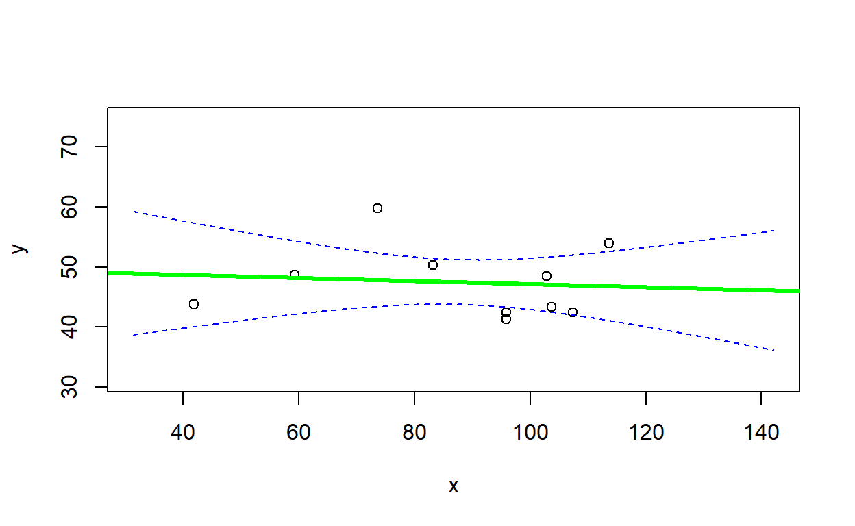
## $fitted_parms
## (Intercept)           x       sigma
## 46.85352516  0.04733444  4.89305075
##
## $slope_in
## [1] FALSE
simdat2 <- LMDataSim(N=100,xlims=c(0,15),parms=c(40,-2.2,1.8) )
LMVerify(simdat2, c(40,-2.2,1.8), plot=T)## `geom_smooth()` using formula = 'y ~ x'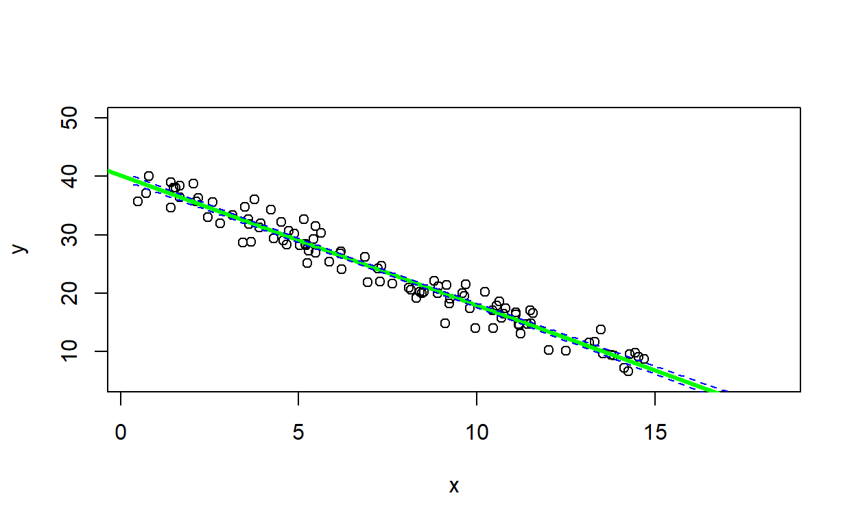
## $fitted_parms
## (Intercept)           x       sigma
##   40.582096   -2.254290    1.865611
##
## $slope_in
## [1] TRUE
Aside: plotting confidence intervals
It is useful to know how to use the ‘predict’ function to compute confidence intervals and prediction intervals for models fitted with ‘lm()’:
   ## this code assumes that 'yourmodel' is fitted with lm!
predict(yourmodel, interval = c("confidence"), level = 0.95)   # for confidence interval
predict(yourmodel, interval = c("prediction"), level = 0.95)   # for prediction interval
Other model objects (fitted with lme4, mgcv, etc.) will have similar ‘predict’ methods, but often will only produce standard errors rather than confidence intervals on predictions..
But otherwise all ‘predict’ methods work in a similar way: the predict function allows you to predict a response (and estimate confidence intervals) for any arbitrary covariate values. To do this you need to add a “newdata” argument to the predict function. For example:
nd <- data.frame(x=seq(lb,ub,length=100))  # note that the predictor names need to match the predictor names in the model object!
predict(yourmodel, newdata=nd, interval = c("confidence"), level = 0.95)   # for confidence interval
Note that the prediction interval code may occasionally return some warnings- which you may safely ignore!
Exercise 2.1c.
Does the 90% confidence interval around the slope estimate (estimated from simulated data with a sample size of 10) contain the “true” slope parameter value 90% of the time? In your WebCampus submission, explain how you addressed this question. Did you need more than 100 simulated data sets to answer this question?
ASIDE: review of conditional statements in R
NOTE: The previous exercise requires the use of “conditional” operations. That is, if a condition is true, do something. If the condition is false, do something else. The syntax for doing this in R is:
if(TRUE){
  do something
}else{
  do something else
}
Let’s say I want to determine the number of vector elements that are cleanly divisible by 3. I could write the following code:
inputvector <- c(1:100) # vector of interest
div_by_three <- 0

for(i in 1:length(inputvector)){
  if(i%%3==0){  # if there is zero remainder after dividing by three
    div_by_three <- div_by_three+1   # then increment the storage variable
  }
}

div_by_three
## [1] 33An alternative way to do this would be to do use the “which()” function. This tells you which indices in a vector correspond to “TRUE” conditions.
For example,
which(c(FALSE,TRUE,TRUE,FALSE))## [1] 2 3Using “which”, we could re-write the above code to take up just one line!
div_by_three <- length(which(inputvector%%3==0))Exercise 2.2: model verification, part 2
How might your results from part 2.1 change if your data simulations DID NOT meet the assumptions of ordinary linear regression- e.g., if the variances were not homogeneous?
To test this, write an R function to generate data that violates a basic assumption regarding the error distribution of standard linear regression. Specifically, your function should generate “heteroskedastic” data, such that the variance of the residuals depends on the magnitude of the mean response value ‘y hat’. For this exercise, you’ll still need to specify a linear relationship (y_hat=ax+b) between your response and predictor - the only difference is that the residual variance is no longer homogeneous. To accomplish this, you need to specify a linear relationship for the standard deviation of residual error as well- this proportional relationship (sd=c*|yhat|) will describe how the residual error changes across the range of your predictor variable.
Some other potential violations of standard assumptions we could also introduce into our data simulations if we wanted to:
- use a non-normal error distribution
- introduce temporal autocorrelation
- introduce other types of correlation structure among the
observations
- use a mixture of two error distributions
- use a non-linear functional form
Exercise 2.2a.
Write a function called “LMDataSim2()” for drawing a set of random observations from a defined linear relationship that meets all the assumptions of ordinary linear regression except for homoskedasticity. This function should be specified as follows:
- input:
- N = an integer specifying the sample size (number of observations to simulate)
- xlims = a vector of length 2 specifying the minimum and maximum
values of the covariate “x”
- parms = a vector of length 3 specifying (in order) the intercept and slope of the relationship between “x” and the expected response (y hat), and a non-negative proportionality constant defining the relationship between the standard deviation of the residuals and y hat (sigma = c*|y_hat|)
- suggested algorithm:
- sample random values (size=“N”) from a uniform distribution (min and
max defined by “xlims”) to represent the covariate (use the “runif()”
function)
- Use the defined linear model (defined by the first two “parms”) to determine the expected value of the response.
- Use the defined linear model (defined by the final value fo ‘parms’) to determine the standard deviation of the response. Note that the standard deviation should now depend on the absolute value (magnitude) of the expected response.
- Add “noise” to the expected values according to the parameters assuming normally distributed residual error (use the “rnorm()” function).
- sample random values (size=“N”) from a uniform distribution (min and
max defined by “xlims”) to represent the covariate (use the “runif()”
function)
- return:
- out = a data frame with number of rows equal to “sample.size”
(number of observations), and two columns:
- the first column, named ‘x’, should represent the values of the “x” variable
- the second column, named ‘y’, should represent the simulated values of the response variable (stochastic observations from the known model defined by “parms”)
- out = a data frame with number of rows equal to “sample.size”
(number of observations), and two columns:
Include your function in your submitted r script!
Test your function- for example, using the following code:
test <- LMDataSim2(500,xlims=c(1,10),parms=c(1,4,.5))
plot(test)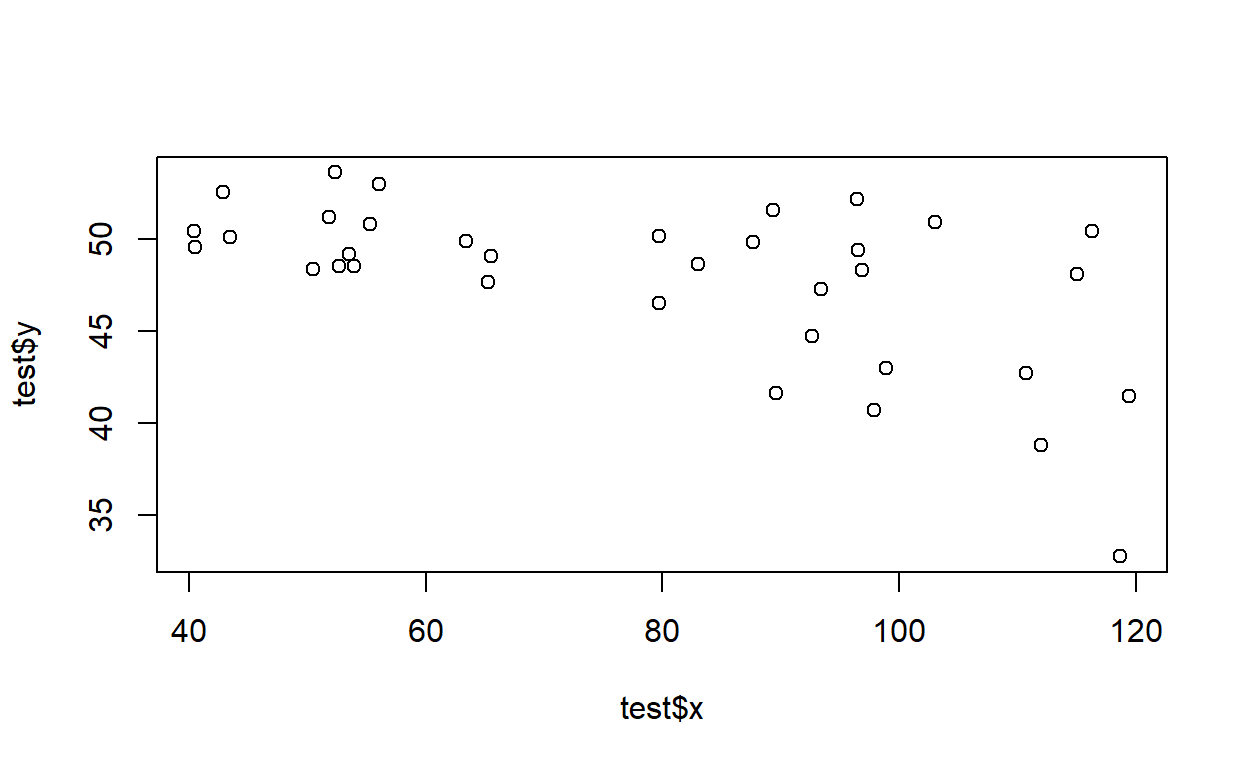
Test your function using the ‘LMVerify’ function you wrote earlier…
simdat <- LMDataSim2(100,xlims=c(1,10),parms=c(3,3,0.3))
LMVerify(simdat, c(3,3,0.3), plot=T)
## `geom_smooth()` using formula = 'y ~ x'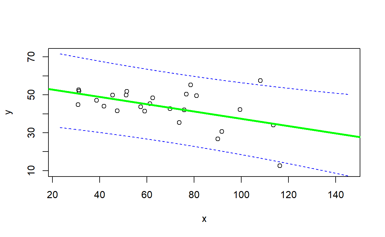
## $fitted_parms
## (Intercept)           x       sigma
##    3.825422    2.821913    6.751277
##
## $slope_in
## [1] TRUE
Exercise 2.2b.
In webcampus, please answer the following question:
Is the estimate of the slope parameter (obtained using the ‘lm()’ function) biased? [note: statistical bias of an estimator is the difference between the estimator’s expected value and the true value of the parameter being estimated]. Ideally, an estimator should be unbiased (bias=0). Briefly explain how you got your answer.
Exercise 2.2c.
In webcampus, please answer the following question:
Is the confidence interval on your estimate of the slope parameter reliable? Is it really a 90% confidence interval?
Exercise 2.2d.
In webcampus, please answer the following question:
Use the figure below to evaluate the goodness-of-fit of a linear regression model (heavy line with prediction interval visualized as dashed lines) fitted to the data (open circles). See the code below for reference about how the figure was generated.
In your written response, please describe how this figure helps you to evaluate goodness-of-fit (i.e., could your observed data have been generated by the model?) What ‘red flags’ might make you think that the linear regression model is not adequate for representing these data?
Finally, briefly describe one scenario (possibly hypothetical) where violation of the heteroskedasticity assumption in linear regression could lead to erroneous inference.
Here is an example of a goodness-of-fit visualization:
##  goodness of fit visualization...

simdat_uv <- LMDataSim2(500,xlims=c(5,120),parms=c(5,5,.25))
mod = lm(y~x, data=simdat_uv)
nd = data.frame(
  x=seq(min(simdat_uv$x),max(simdat_uv$x),length=100)
)
pred = predict(mod,nd,interval="prediction",level=0.89)
plot(simdat_uv)
lines(nd$x, pred[,"fit"],lwd=2)
lines(nd$x, pred[,"lwr"],lwd=1,lty=2)
lines(nd$x, pred[,"upr"],lwd=1,lty=2)
legend("topleft",lty=2,legend="89% prediction interval")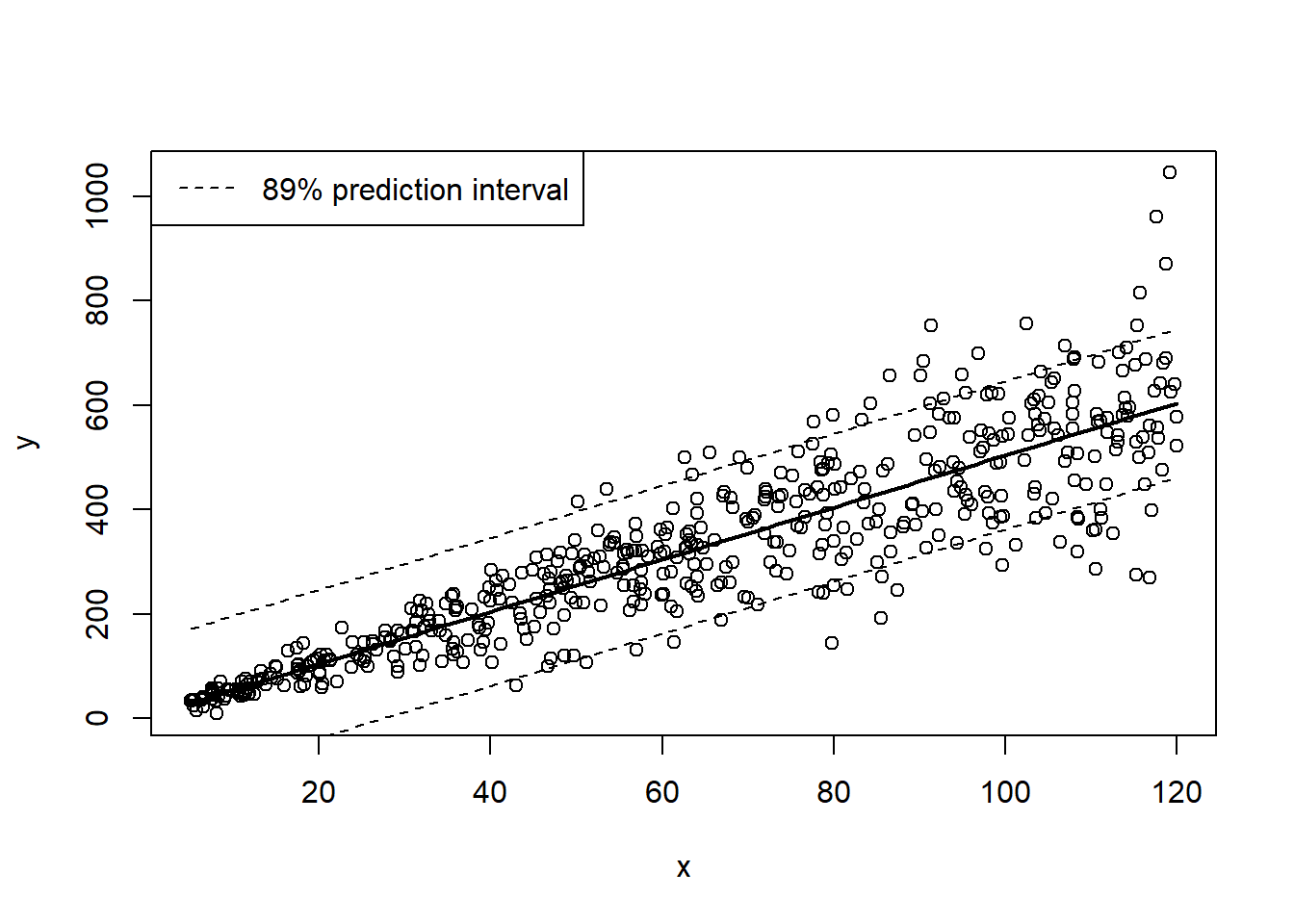
Exercise 2.3: Power analysis!
Review the “power analysis” section of the Data generating model lecture, and complete the following exercises. Recall that we are designing a monitoring program for a population of an at-risk species, and we want to have at least a 75% chance of detecting a decline of 25% or more over a 25 year period. Let’s assume that we are using visual counts, and that the probability of encountering each organism visually is 2% per person-day. The most recent population estimate was 1000 (assume that we know that with certainty).
Exercise 2.3a
Develop a function called “GetPower()” that evaluates the statistical power to detect a decline under user-specified types of monitoring designs (e.g., varying numbers of observers, intervals between successive surveys). This function should be specified as follows:
N0=1000,trend=-0.03,nyears=25,people=1,days=3,survint=2,alpha=0.05
- input:
- N0: initial population abundance (default=1000)
- trend: proportional change in population size each year
(default=-0.03)
- nyears: duration of simulation (in years) (default=25)
- people: number of survey participants each day of each survey year
(default=1)
- days: survey duration, in days (default=3)
- survint: survey interval, in years (e.g., 2 means surveys are conducted every other year) (default=2)
- alpha: maximum acceptable type-I error rate – above which we would be reluctant to conclude that a population is declining.
- suggested algorithm:
- Up to you!!! You can make use of the functions from the “data generation” lecture.
- return:
- A single floating point (real number) value representing the statistical power to detect a decline under the specified default parameters and alpha level. This represents the percent of replicate data sets for which you correctly reject the null hypothesis of “no decline”.
Include your function in your submitted r script!
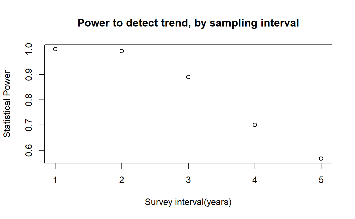
And we can use our new function to do a power analysis:
initabund = 1000
  survints <- c(1:5)
  powers <- numeric(length(survints))
  for(i in 1:length(survints)){
    powers[i] <- GetPower(survint=survints[i])
  }

  plot(powers~survints,xlab="Survey interval(years)",ylab="Statistical Power",main="Power to detect trend, by sampling interval")
Exercise 2.3b.
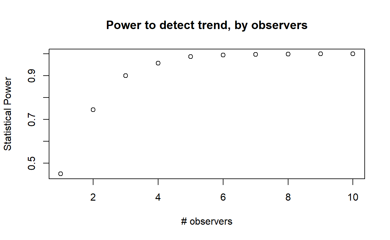
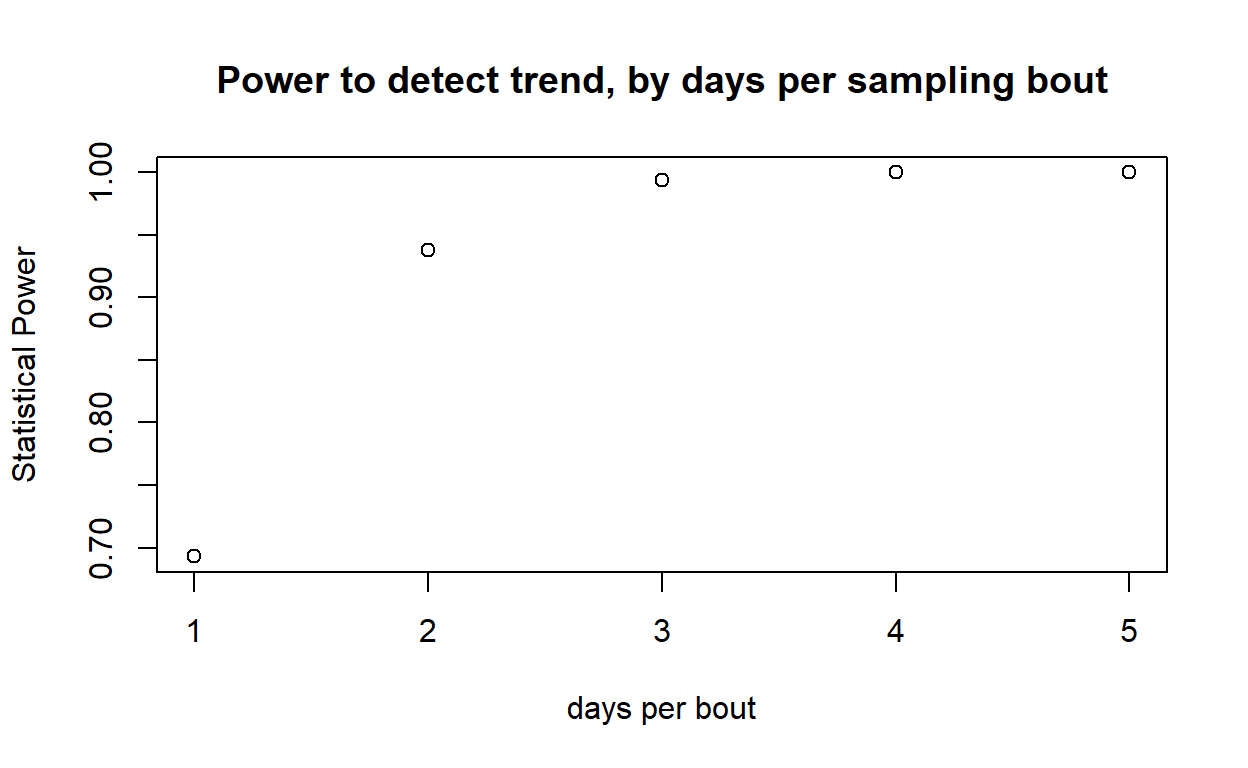
In webcampus, please answer the following question:
For each variable element of the survey design (survey interval, number of observers, days per survey bout), evaluate how statistical power changes across a range of plausible values. Plot out these relationships.
In webcampus, provide ONE of these plots, describe (briefly!) how you produced the plot, and how this information might help managers to develop effective survey protocols for this species.
Exercise 2.3c
Let’s factor in dollar amounts. Let’s assume each observer is paid $200 per day. In addition, let’s assume that the site is fairly remote and it costs $2000 to mount a field expedition (regardless of the number of field technicians). Can you identify a survey strategy to minimize cost while meeting the objective??? What is the optimal survey design in your opinion? Briefly describe how you arrived at this conclusion. [NOTE: don’t overthink this one- you don’t need to find the true optimal solution, just find a solution that meets the objective at relatively low cost and justify your answer!]
CONGRATULATIONS! You have reached the end of lab 2!