Integrated Population Models (IPMs)

Click here to follow along in R: IPM_lecture.R

Introduction

What are IPMs

Integrated population models (IPMs) represent the single, unified analysis of population count data and demographic data.
A statistical method that combines two or more datasets to explore underlying processes and relationships.
An IPM forms joint likelihood between these data sets through with the shared parameter(s) among likelihoods of each data sets.

The Population Part

The goal of population models is to understand the interactions that lead to changes in population size and structure. Population dynamics is the summation of all losses and gains in a population through recruitment, survival, emigration, and immigration. So if population growth rates are changing, there is a change in one of these demographic rates.

The size of a population (N) can be expressed by the following equation: N =S+R+I-E where population size in year t is given by the population size surviving the year before (S), plus the number of new individuals resulting from local recruitment (R) and immigration (I), minus the number of individuals lost as a result of death and emigration (E).

The Integrated Part

An integrated analysis in general is a joint analysis of several datasets on different quantities.Inference is based on the joint likelihood. A key element is that one or several parameters are common in several components of the likelihood but collected independently.

Previous analysis method analyzed these data separately

In IPMS: In these models, all available data are analyzed within a single model; the single data likelihoods are used to create the joint likelihood upon which inference is based.

Stage-Structured (Matrix) Population Models

Most IPMs are based on stage-structured models.Defining the life-cycle graph and demographic rates for your study species a crucial part in the development of a stage-structured population model and for construction of an IPM

Advantages of IPMs

More precise parameter estimates
Incorporates all sources of uncertainty (process variability and sampling processes)
Allows estimation of more demographic quantities (with caution; Riecke et al. 2019)

IPM Components (submodels)

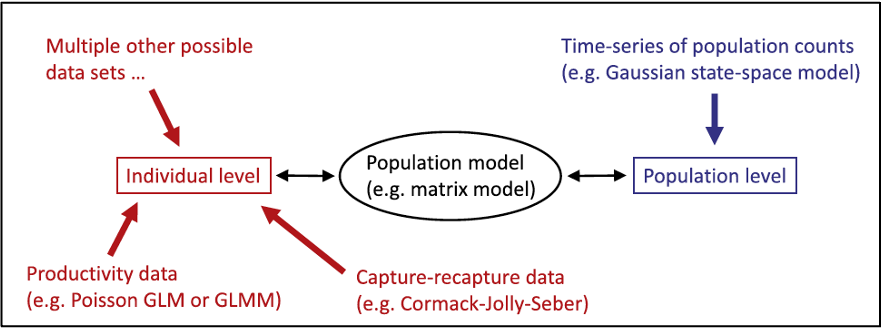
Count data (population level) - Population size surveys

Demographic data (individual level) - Survival surveys - Productivity surveys

This tutorial will briefly review very simplified versions of some (but definitely not all!) potential submodels that are typically included in an IPM.

NOTE: The following examples are borrowed from Schaub and Kery (2022)

Productivity

Reproduction is a key process of any population model. Population models typically require the number of offspring per female and year, which we call “productivity”.

In this example, we show some of the subprocess that make up productivity for birds, but this will not cover all facets of productivity which may look different for different taxa.

Importantly, productivity can be assessed at different stages of the annual cycle.

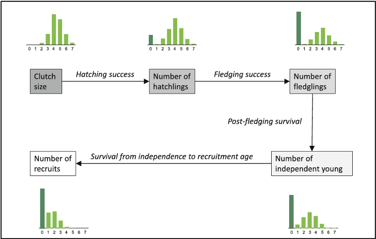
In this example, we will focus on nest survival and brood size.

Nest Survival Models

The primary goal of nest survival models is the estimation of nest success, which is the probability that at least one fledgling is produced by a nest.

Two possible components of nest success:

Incubation
Nestling phase

Data collected for a nest survival study include:

Date of visit
Nest status (alive, inactive)
Optional: age of nest
And more

Data for each nest i are summarized as:

f_i - date when the nest is first detected

j_i - last date the nest was observed as alive

k_i - day when the nest was visited for the last time

x_i - whether the nest was alive during the last visit (fail = 0, success = 1)

Analysis details:

Active nests must be visited repeatedly
Time intervals between visits do not need to be identical
Estimation of daily survival starts on the day when the nest is discovered
The exact date of failure is unknown, unless the nest is observed daily
Date of failure can be estimated from the model, based on daily survival probabilities

In this example, we have nest data on 181 wrynecks from 2002 to 2006 and analyzed by Geiser et al. (2008). Note that dates are recorded such that day 1 is May 16.

First, explore the data

library(IPMbook); library(jagsUI)
data(wryneck)
str(wryneck)

## 'data.frame':    181 obs. of  5 variables:
##  $ f  : int  49 15 23 23 47 11 23 15 65 2 ...
##  $ j  : int  53 32 37 40 66 30 37 30 71 18 ...
##  $ k  : int  53 32 37 40 66 30 37 30 72 18 ...
##  $ x  : int  1 1 1 1 1 1 1 1 0 1 ...
##  $ age: int  16 2 4 2 2 2 5 2 5 2 ...

tail(wryneck)

##      f  j  k x age
## 176  5 25 25 1   1
## 177 53 56 60 0   1
## 178  9 29 29 1   1
## 179 26 46 46 1   1
## 180 55 75 75 1   1
## 181 20 35 35 1   6

As a reading example, nest 177 was detected on day 53 when the nestlings were 1 day old, and it was checked for the last time with nestlings seen alive on day 56. Then, it was checked again on day 60 when the brood was found to have failed (hence, x = 0).

Next, we’ll create daily encounter histories for each nest

# Identify failed broods
fail <- which(wryneck$x==0)
# Create encounter histories
y <- matrix(NA, nrow=length(wryneck$f), ncol=max(wryneck$k))
for (i in 1:length(wryneck$f)){
y[i,wryneck$f[i]] <- 1
y[i,wryneck$j[i]] <- 1
}
for (i in 1:length(fail)){
y[fail[i],wryneck$k[fail[i]]] <- 0
}

View encounter histories of two broods 176 and 177:

y[176,]

##  [1] NA NA NA NA  1 NA NA NA NA NA NA NA NA NA NA NA NA NA NA NA NA NA NA NA  1
## [26] NA NA NA NA NA NA NA NA NA NA NA NA NA NA NA NA NA NA NA NA NA NA NA NA NA
## [51] NA NA NA NA NA NA NA NA NA NA NA NA NA NA NA NA NA NA NA NA NA NA NA NA NA
## [76] NA NA NA NA NA NA

y[177,]

##  [1] NA NA NA NA NA NA NA NA NA NA NA NA NA NA NA NA NA NA NA NA NA NA NA NA NA
## [26] NA NA NA NA NA NA NA NA NA NA NA NA NA NA NA NA NA NA NA NA NA NA NA NA NA
## [51] NA NA  1 NA NA  1 NA NA NA  0 NA NA NA NA NA NA NA NA NA NA NA NA NA NA NA
## [76] NA NA NA NA NA NA

In the encounter history of brood 176 there are NA before the nest was detected and after the nestlings fledged, i.e., the nest was successful. In the model (below) we will define the likelihood in a loop only between the first and last visit and thus NAs outside this loop will not be estimated, nor will they provide any information about daily survival. For nest 177 there are NAs between the last visit when the nest was alive and the visit when the failure was detected, so there is uncertainty about the exact date when the nest failed. The data required to fit the model are these encounter histories, the dates of the first and last visits to each nest, the number of nests and the number of days a brood requires from hatching to fledging (T), which is assumed to be a constant, and is needed to scale daily survival to total nest survival.

We fit a nest survival model where the daily nest survival is a linear function of nestling age. Often daily nest survival increases with nestling age, for instance because nestlings become less sensitive to food shortage, severe weather, or predators. The data bundle contains the age covariables as well as the other needed data and information.

# Bundle data
jags.data <- with(wryneck, list(y=y, f=f, k=k, n.nest=nrow(y), T=21, age=age))
str(jags.data)

## List of 6
##  $ y     : num [1:181, 1:81] NA NA NA NA NA NA NA NA NA NA ...
##  $ f     : int [1:181] 49 15 23 23 47 11 23 15 65 2 ...
##  $ k     : int [1:181] 53 32 37 40 66 30 37 30 72 18 ...
##  $ n.nest: int 181
##  $ T     : num 21
##  $ age   : int [1:181] 16 2 4 2 2 2 5 2 5 2 ...

The likelihood of the nest survival model is similar to that of the Corack-Jolly-Seber model, except that here we assume perfect detection and hence have no observation submodel. As always, the model also has the priors and linear models section where we define our linear models for the primary parameters and the chosen priors. At the end of the code, we compute nest success as a derived parameter that is a function of daily survival and duration T.

# Write JAGS model file
cat(file="model13.txt", "
model {
# Priors and linear models
for (i in 1:n.nest){
for (t in f[i]:(k[i]-1)){
phi[i,t] <- phia[age[i] + t - f[i]]
} #t
} #i
for (a in 1:T){
phia[a] <- ilogit(alpha + beta * a)
}
alpha ~ dnorm(0, 0.001)
beta ~ dnorm(0, 0.001)
# Likelihood
for (i in 1:n.nest){
for (t in (f[i]+1):k[i]){
y[i,t] ~ dbern(phi[i,t-1] * y[i,t-1])
} #t
} #i
# Derived parameter: nest success
nu <- prod(phia[1:T])
}
")
# Initial values
inits <- function(){list(alpha=runif(1, 4, 5), beta=runif(1, 0, 0.1))}
# Parameters monitored
parameters <- c("phia", "nu", "alpha", "beta")
# MCMC settings
ni <- 3000; nb <- 1000; nc <- 3; nt <- 1; na <- 1000
# Call JAGS from R (ART 1 min) and check convergence
out16 <- jags(jags.data, inits, parameters, "model13.txt", n.iter=ni, n.burnin=nb, n.chains=nc,
n.thin=nt, n.adapt=na, parallel=TRUE)

## 
## Processing function input....... 
## 
## Done. 
##  
## Beginning parallel processing using 3 cores. Console output will be suppressed.
## 
## Parallel processing completed.
## 
## Calculating statistics....... 
## 
## Done.

#traceplot(out16) # Not shown
print(out16, 3)

## JAGS output for model 'model13.txt', generated by jagsUI.
## Estimates based on 3 chains of 3000 iterations,
## adaptation = 1000 iterations (sufficient),
## burn-in = 1000 iterations and thin rate = 1,
## yielding 6000 total samples from the joint posterior. 
## MCMC ran in parallel for 0.334 minutes at time 2023-12-06 11:02:30.768117.
## 
##             mean     sd   2.5%     50%   97.5% overlap0     f  Rhat n.eff
## phia[1]    0.971  0.008  0.954   0.972   0.985    FALSE 1.000 1.003   783
## phia[2]    0.974  0.007  0.959   0.974   0.985    FALSE 1.000 1.003   797
## phia[3]    0.976  0.006  0.964   0.976   0.986    FALSE 1.000 1.003   830
## phia[4]    0.978  0.005  0.967   0.978   0.986    FALSE 1.000 1.003   895
## phia[5]    0.979  0.004  0.971   0.980   0.986    FALSE 1.000 1.002  1021
## phia[6]    0.981  0.003  0.974   0.981   0.987    FALSE 1.000 1.002  1272
## phia[7]    0.982  0.003  0.976   0.982   0.988    FALSE 1.000 1.001  1830
## phia[8]    0.984  0.003  0.978   0.984   0.988    FALSE 1.000 1.000  3349
## phia[9]    0.985  0.002  0.980   0.985   0.989    FALSE 1.000 1.000  6000
## phia[10]   0.986  0.002  0.981   0.986   0.990    FALSE 1.000 1.000  6000
## phia[11]   0.987  0.002  0.982   0.987   0.991    FALSE 1.000 1.000  6000
## phia[12]   0.988  0.002  0.983   0.988   0.992    FALSE 1.000 1.000  6000
## phia[13]   0.989  0.002  0.984   0.989   0.993    FALSE 1.000 1.001  3565
## phia[14]   0.989  0.002  0.984   0.990   0.994    FALSE 1.000 1.001  2269
## phia[15]   0.990  0.002  0.985   0.990   0.994    FALSE 1.000 1.001  1674
## phia[16]   0.991  0.003  0.985   0.991   0.995    FALSE 1.000 1.002  1346
## phia[17]   0.991  0.003  0.986   0.992   0.996    FALSE 1.000 1.002  1142
## phia[18]   0.992  0.003  0.986   0.992   0.996    FALSE 1.000 1.003  1006
## phia[19]   0.993  0.003  0.986   0.993   0.997    FALSE 1.000 1.003   908
## phia[20]   0.993  0.003  0.987   0.993   0.997    FALSE 1.000 1.004   835
## phia[21]   0.993  0.003  0.987   0.994   0.997    FALSE 1.000 1.004   779
## nu         0.733  0.036  0.660   0.734   0.801    FALSE 1.000 1.000  6000
## alpha      3.489  0.320  2.899   3.483   4.143    FALSE 1.000 1.005   559
## beta       0.077  0.032  0.016   0.077   0.140    FALSE 0.993 1.004   587
## deviance 111.794 21.447 71.776 110.935 155.855    FALSE 1.000 1.000  5180
## 
## Successful convergence based on Rhat values (all < 1.1). 
## Rhat is the potential scale reduction factor (at convergence, Rhat=1). 
## For each parameter, n.eff is a crude measure of effective sample size. 
## 
## overlap0 checks if 0 falls in the parameter's 95% credible interval.
## f is the proportion of the posterior with the same sign as the mean;
## i.e., our confidence that the parameter is positive or negative.
## 
## DIC info: (pD = var(deviance)/2) 
## pD = 230 and DIC = 341.759 
## DIC is an estimate of expected predictive error (lower is better).

As expected, there is a slight but clear increase with nestling age in the daily nest survival probabilities. The coefficient of age (beta) is positive indicating that nest failure becomes less likely as nestlings get closer to fledging. Overall success during the nestling stage is estimated at 0.73, which means that about three of four nests with hatched young produce at least one fledgling. This model offers great flexibility in modeling all sorts of covariate effects. For example, we can include year effects if the data were collected in different years, and the yearly parameters can be treated as either fixed or random. Individual random effects could also be included, e.g., if some nest boxes were repeatedly occupied and we may want to account for possible nonindependence due to location or parent ID. Daily nest survival could also be modeled as a function of temporalor spatial covariates (e.g., territory quality).

Poisson Models for Brood Size

We will look at two model options for brood size (but there are many other options):

Fit a Poisson GLM to the frequency data
Fit a Poisson GLM to aggregated data

Note: we can fit these two completely separate models inside the same JAGS model statement.

First, we will simulate a brood size data set for illustration:

# Choose constants in simulation
nbrood <- 1000 # Number of broods with young counted
brood.mean <- 1.5 # Average brood size
sd.brood <- 0.3 # log-linear brood random effect
# Draw Poisson random numbers
set.seed(24)
expNyoung <- exp(log(brood.mean) + rnorm(nbrood, 0, sd.brood))
C <- rpois(nbrood, expNyoung)
table(C)

## C
##   0   1   2   3   4   5   6   7   8 
## 231 330 237 134  39  16   7   3   3

We call the count of young “C”. When fitting two models to the same data set in a single JAGS model statement we need to make a copy of that data set.

# Data bundle
jags.data <- list(C1=C, sumC1=sum(C), C1copy=C, nbrood=nbrood)
str(jags.data)

## List of 4
##  $ C1    : int [1:1000] 0 0 1 1 4 1 0 2 0 1 ...
##  $ sumC1 : int 1529
##  $ C1copy: int [1:1000] 0 0 1 1 4 1 0 2 0 1 ...
##  $ nbrood: num 1000

library(jagsUI)

# Write JAGS model file
cat(file="model8.txt", "
model {
# Priors and linear models
rho1 ~ dunif(0, 5) # Mean brood size in model 1
rho2 ~ dunif(0, 5) # Mean brood size in model 2
rho3 ~ dunif(0, 5) # Mean brood size in model 3
tau.rho3 <- pow(sd.rho3, -2)
sd.rho3 ~ dunif(0, 3) # Brood-level overdispersion in model 3
# Likelihoods for three separate models
# Model 1: Poisson GLM for disaggregated data
for (i in 1:nbrood){
C1[i] ~ dpois(rho1)
}
# Model 2: Poisson GLM for aggregated data
sumC1 ~ dpois(rho2 * nbrood)
# Model 3: Poisson GLMM for aggregated data with brood-level overdispersion
for (i in 1:nbrood){
C1copy[i] ~ dpois(pois.mean[i])
log(pois.mean[i]) <- logmean[i]
logmean[i] ~ dnorm(log(rho3), tau.rho3)
}
}
")
# Initial values
inits <- function(){list(rho1=runif(1, 0.5, 2.5), rho2=runif(1, 0.5, 2.5),
rho3=runif(1, 0.5, 2.5))}
# Parameters monitored
parameters <- c("rho1", "rho2", "rho3", "sd.rho3")
# MCMC settings
ni <- 60000; nb <- 10000; nc <- 3; nt <- 10; na <- 1000
# Call JAGS from R (ART 3 min), check convergence and summarize posteriors
out11 <- jags(jags.data, inits, parameters, "model8.txt", n.iter=ni, n.burnin=nb, n.chains=nc,
n.thin=nt, n.adapt=na, parallel=TRUE)

## 
## Processing function input....... 
## 
## Done. 
##  
## Beginning parallel processing using 3 cores. Console output will be suppressed.
## 
## Parallel processing completed.
## 
## Calculating statistics....... 
## 
## Done.

#traceplot(out11) # Not shown
print(out11, 3)

## JAGS output for model 'model8.txt', generated by jagsUI.
## Estimates based on 3 chains of 60000 iterations,
## adaptation = 1000 iterations (sufficient),
## burn-in = 10000 iterations and thin rate = 10,
## yielding 15000 total samples from the joint posterior. 
## MCMC ran in parallel for 2.933 minutes at time 2023-12-06 11:02:51.672964.
## 
##              mean     sd     2.5%      50%    97.5% overlap0 f  Rhat n.eff
## rho1        1.530  0.039    1.454    1.529    1.609    FALSE 1 1.000 15000
## rho2        1.530  0.039    1.453    1.530    1.606    FALSE 1 1.000 15000
## rho3        1.464  0.047    1.372    1.464    1.560    FALSE 1 1.002  1145
## sd.rho3     0.292  0.061    0.138    0.297    0.393    FALSE 1 1.031   156
## deviance 6231.203 44.822 6148.537 6229.101 6330.472    FALSE 1 1.017   202
## 
## Successful convergence based on Rhat values (all < 1.1). 
## Rhat is the potential scale reduction factor (at convergence, Rhat=1). 
## For each parameter, n.eff is a crude measure of effective sample size. 
## 
## overlap0 checks if 0 falls in the parameter's 95% credible interval.
## f is the proportion of the posterior with the same sign as the mean;
## i.e., our confidence that the parameter is positive or negative.
## 
## DIC info: (pD = var(deviance)/2) 
## pD = 994.6 and DIC = 7225.823 
## DIC is an estimate of expected predictive error (lower is better).

Some other models for brood size include:

Zero-inflated normal or Poisson
Poisson with truncation
Poisson with censoring
Poisson log-normal model GLMM (for a brood effect)

Survival Models

Cormack-Jolly-Seber Model for Capture-Recapture Data

First, simulate a data set

# Choose values for data simulation
nmarked <- 10 # Number of marked individuals at each occasion
nyears <- 11 # Number of years
phi <- 0.8 # Constant apparent survival probability
p <- 0.4 # Constant recapture probability

An individual first caught on the last year of the study has no opportunity of being recaptured during the study. Such individuals do not carry any information about survival and can be discarded from the analysis. So in our simulation, we choose first-capture occasions only up to the penultimate year.

# Determine occasion when an individual first captured and marked
f <- rep(1:(nyears-1), each=nmarked)
nind <- length(f) # Total number of marked individuals
# State or ecological process
z <- array(NA, dim=c(nind, nyears)) # Empty alive/dead matrix
# Initial conditions: all individuals alive at f(i)
for (i in 1:nind){
z[i,f[i]] <- 1
}
set.seed(1) # Initialize the RNGs in R
# Propagate alive/dead process forwards via transition rule:
# Alive individuals survive with probability phi
for (i in 1:nind){
for (t in (f[i]+1):nyears){
z[i,t] <- rbinom(1, 1, z[i,t-1] * phi)
} #t
} #i
head(z); tail(z) # look at start and end of z

##      [,1] [,2] [,3] [,4] [,5] [,6] [,7] [,8] [,9] [,10] [,11]
## [1,]    1    1    1    1    0    0    0    0    0     0     0
## [2,]    1    1    0    0    0    0    0    0    0     0     0
## [3,]    1    0    0    0    0    0    0    0    0     0     0
## [4,]    1    1    1    1    1    1    1    1    1     1     1
## [5,]    1    0    0    0    0    0    0    0    0     0     0
## [6,]    1    1    1    0    0    0    0    0    0     0     0

##        [,1] [,2] [,3] [,4] [,5] [,6] [,7] [,8] [,9] [,10] [,11]
##  [95,]   NA   NA   NA   NA   NA   NA   NA   NA   NA     1     1
##  [96,]   NA   NA   NA   NA   NA   NA   NA   NA   NA     1     1
##  [97,]   NA   NA   NA   NA   NA   NA   NA   NA   NA     1     1
##  [98,]   NA   NA   NA   NA   NA   NA   NA   NA   NA     1     1
##  [99,]   NA   NA   NA   NA   NA   NA   NA   NA   NA     1     1
## [100,]   NA   NA   NA   NA   NA   NA   NA   NA   NA     1     1

# Observation process: simulate observations
y <- array(0, dim=c(nind, nyears))
for (i in 1:nind){
y[i,f[i]] <- 1
for(t in (f[i]+1):nyears){
y[i,t] <- rbinom(1, 1, z[i,t] * p)
} #t
} #i

head(y) # Complete simulated capture-recapture data set

##      [,1] [,2] [,3] [,4] [,5] [,6] [,7] [,8] [,9] [,10] [,11]
## [1,]    1    0    1    0    0    0    0    0    0     0     0
## [2,]    1    1    0    0    0    0    0    0    0     0     0
## [3,]    1    0    0    0    0    0    0    0    0     0     0
## [4,]    1    0    1    0    1    0    0    0    1     0     0
## [5,]    1    0    0    0    0    0    0    0    0     0     0
## [6,]    1    1    0    0    0    0    0    0    0     0     0

for (i in 1:10){ # Look at true and observed states of first 10 individuals
print(rbind("True state (z)" = z[i,], "Observed state (y)" = y[i,]))
browser()
}

##                    [,1] [,2] [,3] [,4] [,5] [,6] [,7] [,8] [,9] [,10] [,11]
## True state (z)        1    1    1    1    0    0    0    0    0     0     0
## Observed state (y)    1    0    1    0    0    0    0    0    0     0     0
## Called from: eval(expr, envir, enclos)
## debug at <text>#3: print(rbind(`True state (z)` = z[i, ], `Observed state (y)` = y[i, 
##     ]))
##                    [,1] [,2] [,3] [,4] [,5] [,6] [,7] [,8] [,9] [,10] [,11]
## True state (z)        1    1    0    0    0    0    0    0    0     0     0
## Observed state (y)    1    1    0    0    0    0    0    0    0     0     0
## debug at <text>#4: browser()
## debug at <text>#3: print(rbind(`True state (z)` = z[i, ], `Observed state (y)` = y[i, 
##     ]))
##                    [,1] [,2] [,3] [,4] [,5] [,6] [,7] [,8] [,9] [,10] [,11]
## True state (z)        1    0    0    0    0    0    0    0    0     0     0
## Observed state (y)    1    0    0    0    0    0    0    0    0     0     0
## debug at <text>#4: browser()
## debug at <text>#3: print(rbind(`True state (z)` = z[i, ], `Observed state (y)` = y[i, 
##     ]))
##                    [,1] [,2] [,3] [,4] [,5] [,6] [,7] [,8] [,9] [,10] [,11]
## True state (z)        1    1    1    1    1    1    1    1    1     1     1
## Observed state (y)    1    0    1    0    1    0    0    0    1     0     0
## debug at <text>#4: browser()
## debug at <text>#3: print(rbind(`True state (z)` = z[i, ], `Observed state (y)` = y[i, 
##     ]))
##                    [,1] [,2] [,3] [,4] [,5] [,6] [,7] [,8] [,9] [,10] [,11]
## True state (z)        1    0    0    0    0    0    0    0    0     0     0
## Observed state (y)    1    0    0    0    0    0    0    0    0     0     0
## debug at <text>#4: browser()
## debug at <text>#3: print(rbind(`True state (z)` = z[i, ], `Observed state (y)` = y[i, 
##     ]))
##                    [,1] [,2] [,3] [,4] [,5] [,6] [,7] [,8] [,9] [,10] [,11]
## True state (z)        1    1    1    0    0    0    0    0    0     0     0
## Observed state (y)    1    1    0    0    0    0    0    0    0     0     0
## debug at <text>#4: browser()
## debug at <text>#3: print(rbind(`True state (z)` = z[i, ], `Observed state (y)` = y[i, 
##     ]))
##                    [,1] [,2] [,3] [,4] [,5] [,6] [,7] [,8] [,9] [,10] [,11]
## True state (z)        1    1    1    1    1    1    1    1    0     0     0
## Observed state (y)    1    1    1    0    0    0    1    0    0     0     0
## debug at <text>#4: browser()
## debug at <text>#3: print(rbind(`True state (z)` = z[i, ], `Observed state (y)` = y[i, 
##     ]))
##                    [,1] [,2] [,3] [,4] [,5] [,6] [,7] [,8] [,9] [,10] [,11]
## True state (z)        1    1    1    1    1    1    0    0    0     0     0
## Observed state (y)    1    0    0    0    1    0    0    0    0     0     0
## debug at <text>#4: browser()
## debug at <text>#3: print(rbind(`True state (z)` = z[i, ], `Observed state (y)` = y[i, 
##     ]))
##                    [,1] [,2] [,3] [,4] [,5] [,6] [,7] [,8] [,9] [,10] [,11]
## True state (z)        1    1    1    1    1    1    0    0    0     0     0
## Observed state (y)    1    0    0    0    1    1    0    0    0     0     0
## debug at <text>#4: browser()
## debug at <text>#3: print(rbind(`True state (z)` = z[i, ], `Observed state (y)` = y[i, 
##     ]))
##                    [,1] [,2] [,3] [,4] [,5] [,6] [,7] [,8] [,9] [,10] [,11]
## True state (z)        1    1    1    1    1    1    1    1    1     1     1
## Observed state (y)    1    0    0    1    1    0    1    0    0     1     0
## debug at <text>#4: browser()

We can now fit the simplest possible CJS model in JAGS for illustration. For the data bundle, we need to provide the capture-recapture data matrix, its dimensions and the vector f that indicates the marking occasion for each individual.

# Data bundle
jags.data <- list(y=y, f=f, nind=nind, nyears=ncol(y))
str(jags.data)

## List of 4
##  $ y     : num [1:100, 1:11] 1 1 1 1 1 1 1 1 1 1 ...
##  $ f     : int [1:100] 1 1 1 1 1 1 1 1 1 1 ...
##  $ nind  : int 100
##  $ nyears: int 11

We develop the SSM to fit the CJS model to the data. The likelihood of the model is written in the most general way, that is, apparent survival and recapture are defined as two matrices with elements indexed by i and t. Hence, both parameters could vary among individuals and over time. To fit a model with constant rates, we specify a linear model where we assign the same two constants (phi.const and p.const) to each element in the two parameter matrices and then place priors on these parameters.

# Write JAGS model file
cat(file="model14.txt", "
model {
# Priors and linear models
phi.const ~ dunif(0, 1) # Vague prior for constant phi
p.const ~ dunif(0, 1) # Vague prior for constant p
for (i in 1:nind){ # Loop over individuals
for (t in f[i]:(nyears-1)){ # Loop over time intervals/occasions
phi[i,t] <- phi.const # Here we model pattern in phi ...
p[i,t] <- p.const # ... and p
} #t
} #i
# Likelihood
for (i in 1:nind){
# Define latent state at first capture
z[i,f[i]] <- 1
for (t in (f[i]+1):nyears){
# State process
z[i,t] ~ dbern(z[i,t-1] * phi[i,t-1])
# Observation process
y[i,t] ~ dbern(z[i,t] * p[i,t-1])
} #t
} #i
}
")

# Initial values
inits <- function(){list(z=zInit(y))}

# Parameters monitored
parameters <- c("phi.const", "p.const") # Could also add "z"
# MCMC settings
ni <- 3000; nb <- 1000; nc <- 3; nt <- 1; na <- 1000
# Call JAGS from R (ART < 1 min) and check convergence
out17 <- jags(jags.data, inits, parameters, "model14.txt", n.iter=ni, n.burnin=nb, n.chains=nc,
n.thin=nt, n.adapt=na, parallel=TRUE)

## 
## Processing function input....... 
## 
## Done. 
##  
## Beginning parallel processing using 3 cores. Console output will be suppressed.
## 
## Parallel processing completed.
## 
## Calculating statistics....... 
## 
## Done.

#traceplot(out17) # Not shown
print(out17, 3)

## JAGS output for model 'model14.txt', generated by jagsUI.
## Estimates based on 3 chains of 3000 iterations,
## adaptation = 1000 iterations (sufficient),
## burn-in = 1000 iterations and thin rate = 1,
## yielding 6000 total samples from the joint posterior. 
## MCMC ran in parallel for 0.072 minutes at time 2023-12-06 11:05:48.632437.
## 
##              mean     sd    2.5%     50%   97.5% overlap0 f  Rhat n.eff
## phi.const   0.830  0.028   0.774   0.830   0.884    FALSE 1 1.002   834
## p.const     0.414  0.038   0.341   0.414   0.490    FALSE 1 1.001  1567
## deviance  401.296 19.561 365.917 400.106 441.370    FALSE 1 1.004   539
## 
## Successful convergence based on Rhat values (all < 1.1). 
## Rhat is the potential scale reduction factor (at convergence, Rhat=1). 
## For each parameter, n.eff is a crude measure of effective sample size. 
## 
## overlap0 checks if 0 falls in the parameter's 95% credible interval.
## f is the proportion of the posterior with the same sign as the mean;
## i.e., our confidence that the parameter is positive or negative.
## 
## DIC info: (pD = var(deviance)/2) 
## pD = 190.7 and DIC = 591.964 
## DIC is an estimate of expected predictive error (lower is better).

We must provide initial values for the latent states z that do not contradict either the model or the data because otherwise JAGS will crash. The function zInit in the IPMbook package generates such initial values for single-state capture-recapture data.

This model requires some homogeneity assumptions. For example, in our model we assume that survival and recapture is identical for all individuals and occasions. In life encounter data some behaviors of the marked individuals can lead to the violation of the homogeneity assumptions. For instance, when some individuals are not really part of the marked population, but are mere transients, i.e., appear only during one occasion and then are gone. Their apparent survival is effectively zero. Another problematic type of behavior may affect capture. Depending on the sampling protocol, some individuals may become trap-happy or trap-shy after an earlier capture, i.e., their capture probability changes after they are captured once or more times.

Survival and recapture can both be modeled as a function of covariates or with random effects by appropriate specification of linear models.

State-Space Model for Population Counts

State-space models are used to analyze time-series data where the true state (e.g., population size) of a system is believed to be unobservable, but can be indirectly observed through noisy measurements.

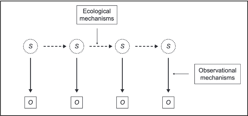
State-space models use an observed time series of counts (or other observed responses) and decompose them into: 1) Process variation 2) Observation error

Example using the exponential population model:

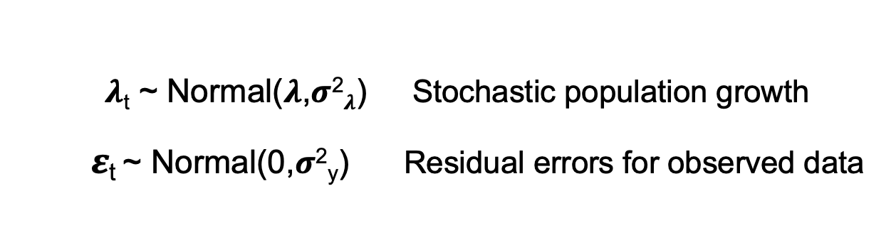
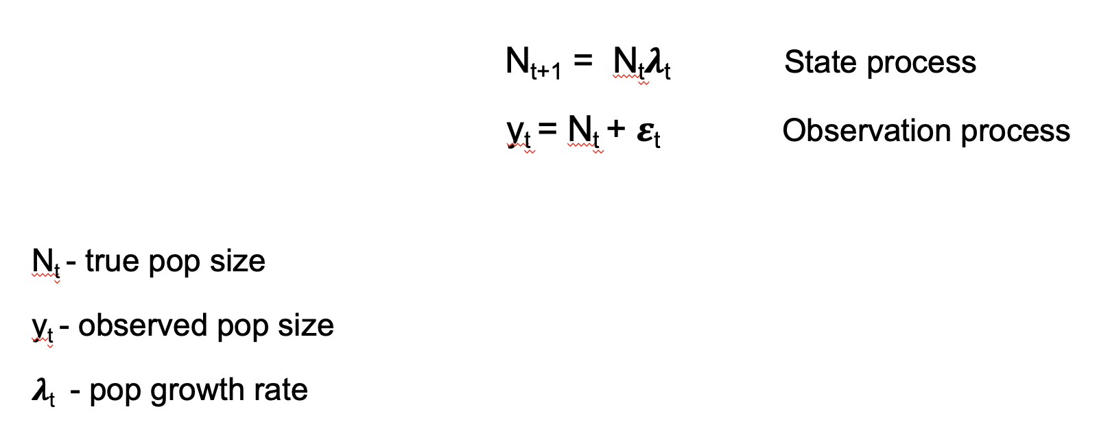Stochasticity is included in the model by making two distributional assumptions about the population growth rate and the observation errors

First, simulate a data set of population sizes and observations

# Chose constants
nyears <- 25            # Number of years
N1 <- 30                # Initial population size, t=1 
mu.lam <- 1.02          # Mean annual population growth rate
sig2.lam <- 0.02        # Process (temporal) variation of the growth rate
sig2.y <- 400           # Variance of the observation error

# Simulate true system state
N <- numeric(nyears)
N[1] <- N1                     # Set initial abundance
set.seed(1)
lambda <- rnorm(nyears-1, mu.lam,sqrt(sig2.lam))   # Draw random lambdas
for(t in 1:(nyears-1)){     
  N[t+1] <- N[t]*lambda[t]     # Propagate population size forward
}

# Simulate observations
eps <- rnorm(nyears,0,sqrt(sig2.y))   # Draw random residuals 
y <- N + eps                   # Add residual error to value of true state

Fit the data-generating model in JAGS

library(IPMbook); library(jagsUI)
# Data bundle
jags.data <- list(y=y, T=length(y))
str(jags.data)

## List of 2
##  $ y: num [1:25] 42.4 26.82 26.11 -3.06 23.27 ...
##  $ T: int 25

# Write JAGS model file
cat(file="model1.txt", "
model {
# Priors and linear models
mu.lam ~ dunif(0, 10) # Prior for mean growth rate
sig.lam ~ dunif(0, 1) # Prior for sd of growth rate
sig2.lam <- pow(sig.lam, 2)
tau.lam <- pow(sig.lam, -2)
sig.y ~ dunif(0.1, 100) # Prior for sd of observation process
sig2.y <- pow(sig.y, 2)
tau.y <- pow(sig.y, -2)
# Likelihood
# Model for the initial population size: uniform priors
N[1] ~ dunif(0, 500)
# Process model over time: our model of population dynamics
for (t in 1:(T-1)){
lambda[t] ~ dnorm(mu.lam, tau.lam)
N[t+1] <- N[t] * lambda[t]
}
# Observation process
for (t in 1:T){
y[t] ~ dnorm(N[t], tau.y)
}
}
")
# Initial values
inits <- function(){list(sig.lam=runif(1, 0, 1))}
# Parameters monitored
parameters <- c("lambda", "mu.lam", "sig2.y", "sig2.lam", "sig.y", "sig.lam", "N")
# MCMC settings
ni <- 200000; nb <- 10000; nc <- 3; nt <- 100; na <- 5000
# Call JAGS from R (ART <1 min), check convergence and summarize posteriors
out1 <- jags(jags.data, inits, parameters, "model1.txt", n.iter=ni, n.burnin=nb, n.chains=nc,
n.thin=nt, n.adapt=na, parallel=TRUE)

## 
## Processing function input....... 
## 
## Done. 
##  
## Beginning parallel processing using 3 cores. Console output will be suppressed.
## 
## Parallel processing completed.
## 
## Calculating statistics....... 
## 
## Done.

#traceplot(out1) # Not shown
print(out1, 3)

## JAGS output for model 'model1.txt', generated by jagsUI.
## Estimates based on 3 chains of 2e+05 iterations,
## adaptation = 5000 iterations (sufficient),
## burn-in = 10000 iterations and thin rate = 100,
## yielding 5700 total samples from the joint posterior. 
## MCMC ran in parallel for 0.212 minutes at time 2023-12-06 11:05:53.579164.
## 
##               mean      sd    2.5%     50%   97.5% overlap0     f  Rhat n.eff
## lambda[1]    0.999   0.166   0.566   1.032   1.286    FALSE 1.000 1.017  3747
## lambda[2]    1.018   0.169   0.659   1.036   1.342    FALSE 1.000 1.042  1061
## lambda[3]    0.988   0.261   0.507   1.038   1.290    FALSE 0.978 1.210    68
## lambda[4]    1.107   0.185   0.869   1.062   1.578    FALSE 1.000 1.047   547
## lambda[5]    1.071   0.343   0.774   1.067   1.550    FALSE 0.978 1.240    61
## lambda[6]    1.110   0.186   0.867   1.064   1.587    FALSE 1.000 1.068   241
## lambda[7]    1.023   0.161   0.661   1.038   1.308    FALSE 1.000 1.050   877
## lambda[8]    1.059   0.155   0.793   1.047   1.406    FALSE 1.000 1.046   973
## lambda[9]    1.026   0.158   0.692   1.040   1.297    FALSE 1.000 1.058   688
## lambda[10]   1.004   0.161   0.619   1.033   1.260    FALSE 1.000 1.030  5700
## lambda[11]   1.098   0.166   0.862   1.061   1.518    FALSE 1.000 1.045   614
## lambda[12]   1.086   0.155   0.849   1.058   1.468    FALSE 1.000 1.041   890
## lambda[13]   1.075   0.148   0.834   1.055   1.405    FALSE 1.000 1.057  1396
## lambda[14]   1.072   0.146   0.827   1.054   1.415    FALSE 1.000 1.038  1737
## lambda[15]   1.036   0.134   0.753   1.043   1.315    FALSE 1.000 1.028  5700
## lambda[16]   1.002   0.143   0.646   1.032   1.240    FALSE 1.000 1.018  5219
## lambda[17]   1.054   0.141   0.795   1.047   1.362    FALSE 1.000 1.041  1585
## lambda[18]   1.108   0.157   0.889   1.069   1.517    FALSE 1.000 1.029   589
## lambda[19]   1.068   0.137   0.820   1.054   1.390    FALSE 1.000 1.029  5700
## lambda[20]   1.023   0.136   0.699   1.041   1.259    FALSE 1.000 1.028  3343
## lambda[21]   1.089   0.131   0.871   1.063   1.416    FALSE 1.000 1.026   971
## lambda[22]   1.138   0.159   0.949   1.089   1.536    FALSE 1.000 1.037   405
## lambda[23]   1.075   0.121   0.863   1.057   1.363    FALSE 1.000 1.024  2010
## lambda[24]   0.946   0.158   0.557   1.000   1.152    FALSE 1.000 1.010   482
## mu.lam       1.052   0.044   0.979   1.050   1.146    FALSE 1.000 1.047  2648
## sig2.y     252.174 114.299 101.566 232.740 515.859    FALSE 1.000 1.037   363
## sig2.lam     0.036   0.095   0.000   0.009   0.230    FALSE 1.000 1.265    58
## sig.y       15.545   3.245  10.078  15.256  22.713    FALSE 1.000 1.014   502
## sig.lam      0.131   0.137   0.004   0.094   0.480    FALSE 1.000 1.118    95
## N[1]        28.375   8.684  15.005  27.137  49.269    FALSE 1.000 1.013  1355
## N[2]        27.490   6.616  15.509  27.157  42.382    FALSE 1.000 1.003  5700
## N[3]        27.505   6.176  16.037  27.284  40.117    FALSE 1.000 1.006  5700
## N[4]        26.778   8.285  12.602  27.597  39.152    FALSE 0.978 1.131    83
## N[5]        28.960   8.679  14.969  29.782  40.813    FALSE 0.978 1.170    73
## N[6]        32.647   6.532  19.621  32.722  45.318    FALSE 1.000 1.034   244
## N[7]        35.776   7.600  23.020  35.116  53.295    FALSE 1.000 1.011   504
## N[8]        35.903   6.413  23.629  35.855  48.937    FALSE 1.000 1.015   435
## N[9]        37.632   6.689  25.094  37.385  51.838    FALSE 1.000 1.011   630
## N[10]       38.112   6.486  25.334  38.158  51.099    FALSE 1.000 1.014  1135
## N[11]       37.781   6.502  23.480  38.427  49.226    FALSE 1.000 1.011   448
## N[12]       40.905   6.297  27.972  41.196  52.896    FALSE 1.000 1.014   858
## N[13]       43.950   6.395  31.581  43.881  56.847    FALSE 1.000 1.013  2164
## N[14]       46.793   6.642  33.970  46.622  60.496    FALSE 1.000 1.013  3536
## N[15]       49.709   7.101  37.057  49.205  65.792    FALSE 1.000 1.006  5700
## N[16]       51.056   7.073  37.603  50.808  66.181    FALSE 1.000 1.010  4432
## N[17]       50.634   7.313  34.256  51.447  63.056    FALSE 1.000 1.010   558
## N[18]       52.880   7.427  36.231  53.615  65.888    FALSE 1.000 1.008   662
## N[19]       57.905   7.266  42.750  57.924  72.581    FALSE 1.000 1.004  2647
## N[20]       61.358   7.885  45.966  61.286  77.094    FALSE 1.000 1.010  3347
## N[21]       62.196   8.034  44.798  62.780  76.457    FALSE 1.000 1.008   874
## N[22]       67.163   7.916  51.162  67.409  81.801    FALSE 1.000 1.009  2917
## N[23]       75.876   9.718  58.065  75.038  96.587    FALSE 1.000 1.006  1758
## N[24]       81.263  11.844  60.520  79.851 108.812    FALSE 1.000 1.003  1123
## N[25]       75.812  11.600  51.972  76.174  97.962    FALSE 1.000 1.007  1147
## deviance   206.085   7.136 189.226 206.742 218.797    FALSE 1.000 1.022   367
## 
## **WARNING** Rhat values indicate convergence failure. 
## Rhat is the potential scale reduction factor (at convergence, Rhat=1). 
## For each parameter, n.eff is a crude measure of effective sample size. 
## 
## overlap0 checks if 0 falls in the parameter's 95% credible interval.
## f is the proportion of the posterior with the same sign as the mean;
## i.e., our confidence that the parameter is positive or negative.
## 
## DIC info: (pD = var(deviance)/2) 
## pD = 25.3 and DIC = 231.417 
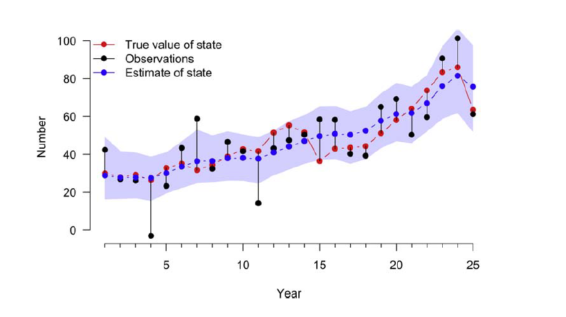
## DIC is an estimate of expected predictive error (lower is better).

We see in the figure below, the estimates do a pretty good job recovering the input values, i.e., the true states. Note that the credible interval refers to the true state and not to the observations so we don’t need to worry about a number of counts that lie outside the blue band.

Building IPMS

Now that you’ve learned about matrix models and seen multiple examples of the sub-models that create in IPM in the JAGS language, how do you bring them together?

First Step: Develop a (matrix) model that links population sizes and specify your known demographic rates. This was your Leslie matrix.
Second Step: Formulate the likelihood for each available data set (submodel) separately.
Third Step: The joint likelihood of all datasets combined must be created. This is the likelihood on which inference is based.

That will be most of our lab on Monday!

Resources for learning about IPMs

Paper: Integrated population models: a novel analysis framework for deeper insights into population dynamics by Michael Schaub & Fitsum Abadi (2011) view

Paper: Integrated population models: Model assumptions and inference by Riecke et al. (2019) view

Textbook: Integrated Population Models by Michael Schaub and Marc Kery (2022)