Understanding Random Intercepts and Slopes in Mixed-Effects Models using lme4 and glmmTMB

Background

Multi-level regression, also known as a hierarchical linear model, is a statistical technique used to analyse data with a hierarchical, nested, or clustered structure, such as students within classrooms or employees within companies. It extends standard regression by accounting for the fact that observations from the same group are not independent, allowing for differences in intercepts and slopes across groups. This approach acknowledges the data structure, prevents biased standard errors, and allows examination of effects at different levels. Real-world data often have hierarchical or repeated structures, and ignoring grouping leads to biased estimates and underestimated uncertainty. Mixed models allow for group-specific variation, partial pooling, and better generalization across groups.

Why multi-levels matter

Data from the same class will perform more similarly than data from different contexts.
- Children in the same class will perform more similarly than children from different classes, potentially because they have the same teacher and use the same materials.
- People treated in the same clinics should be more similar in their responses than those treated at different clinics, even if they use the same protocols, etc.
Lack of Independence
- Violates the assumption of errors being independent
- Bias, SEs, CIs, and p-values

Fixed vs Random Effects

Fixed effects represent population-level parameters that estimate specific coefficients applicable to the entire dataset, such as treatment effects or time trends. In contrast, random effects capture group-level variation by modeling variance components that reflect how individual groups, like schools, subjects, or sites, deviate from the overall average. While fixed effects provide estimates of average trends, random effects account for the variability among groups, allowing for partial pooling and more accurate inference.

Nested vs Crossed Random Effects

Nested: One factor is contained within another Syntax: (1 | school/classroom)
Crossed: Factors interact independently Syntax: (1 | student) + (1 | teacher)

Benefits of multi-level models

Modelling variability in effects across contexts (quantify variation among groups)
- Model the variability in intercepts
- Model the variability in slopes
Gives more realistic predictions (we don’t force every group to behave identically)
Reduces bias in estimated effects and standard errors.

Mixed-effects models are used when data are grouped or clustered. For example, students nested within schools, patients measured by different doctors, or repeated measures on individuals over time.

These models allow us to:

Model population-level effects (fixed effects): e.g., the overall effect of treatment.
Model group-level variation (random effects): e.g., how the treatment effect or baseline differs across different groups.

These characteristics makes them particularly valuable when we expect differences among groups but want to share information across them.

When to use which?

Scenario	Recommended Package
Simple Gaussian or Poisson GLMM	lme4
Zero-inflated or overdispersed counts	glmmTMB
Need for hurdle or beta models	glmmTMB
Fast prototyping with standard families	lme4
Diagnostics with simulated residuals	glmmTMB + DHARMa

We will focus on lmer to explain random slopes and intercepts

Random Intercepts and Random Slopes

When we fit a mixed-effects model using lmer, we can include random intercepts and random slopes.

Random intercept: Each group has its own baseline outcome.
Random slope: Each group can differ in how strongly a predictor (like treatment) affects the outcome.

Mathematically:

\[ y_{ij} = (\beta_0 + u_{0j}) + (\beta_1 + u_{1j})x_{ij} + \epsilon_{ij} \]

Where:

$\beta_0$, $\beta_1$ = fixed (overall) intercept and slope
$u_{0j}$, $u_{1j}$ = random deviations for group j
$\epsilon_{ij}$ = residual error

Syntax in `lme4`

Model Type	Formula	Meaning
Random intercept only	`(1 \| group)`	Groups have different intercepts
Random intercept and slope	`(1 + treatment \| group)`	Groups have different intercepts and treatment effects
Crossed random effects	`(1 + treatment \| A) + (1 \| B)`	Effects vary across two independent grouping factors

Correlation Between Intercepts and Slopes

When we specify (1 + treatment | group), the model also estimates how correlated the random intercepts and slopes are.

\[ \rho = \frac{\sigma_{u_0, u_1}}{\sigma_{u_0} \sigma_{u_1}} \]

The estimated correlation can ether be positive or negative.

A positive correlation means schools with higher intercepts also tend to have stronger treatment effects.
A negative correlation means schools with higher intercepts tend to have smaller treatment effects.

Let us work through examples for nested and crossed random effects

We will do the following

Go through data simulation for running both model types
Extract and interpret results
Brace up for a real data. It’s going to be fun

Workflow 1: Nested Random Effects (Schools and Students)

We’ll simulate a dataset where students are nested within schools, and each school has its own baseline and treatment effect. Look at this as students inside school.
We are working with two hypothetical treatments namely control and treated.
control and treated can be interpreted as two distinct sets of students (e.g., male vs female; undergraduate vs graduate, etc)

knitr::opts_chunk$set(echo = TRUE)

library(lme4)

## Loading required package: Matrix

library(glmmTMB)
library(tidyverse)

## ── Attaching core tidyverse packages ──────────────────────── tidyverse 2.0.0 ──
## ✔ dplyr     1.1.4     ✔ readr     2.1.5
## ✔ forcats   1.0.0     ✔ stringr   1.5.1
## ✔ ggplot2   4.0.0     ✔ tibble    3.3.0
## ✔ lubridate 1.9.4     ✔ tidyr     1.3.1
## ✔ purrr     1.1.0

## ── Conflicts ────────────────────────────────────────── tidyverse_conflicts() ──
## ✖ tidyr::expand() masks Matrix::expand()
## ✖ dplyr::filter() masks stats::filter()
## ✖ dplyr::lag()    masks stats::lag()
## ✖ tidyr::pack()   masks Matrix::pack()
## ✖ tidyr::unpack() masks Matrix::unpack()
## ℹ Use the conflicted package (<http://conflicted.r-lib.org/>) to force all conflicts to become errors

library(ggplot2)
library(dplyr)
library(broom.mixed)

1.1 Data Generation for Nested Model

set.seed(123)
n_schools <- 5
n_students <- 50

df_nested <- data.frame(
  school = factor(rep(1:n_schools, each = n_students)),
  treatment = factor(rep(rep(c("control","treated"), each = n_students/2), times = n_schools))
)

# Random intercepts and slopes per school
school_intercepts <- rnorm(n_schools, 0, 1)
school_slopes <- rnorm(n_schools, 2, 0.5)

df_nested$y <- 10 +
  school_intercepts[as.numeric(df_nested$school)] +
  school_slopes[as.numeric(df_nested$school)] * (df_nested$treatment == "treated") +
  rnorm(nrow(df_nested), 0, 1)

head(df_nested)

##   school treatment         y
## 1      1   control 10.663606
## 2      1   control  9.799338
## 3      1   control  9.840296
## 4      1   control  9.550207
## 5      1   control  8.883683
## 6      1   control 11.226437

str(df_nested)

## 'data.frame':    250 obs. of  3 variables:
##  $ school   : Factor w/ 5 levels "1","2","3","4",..: 1 1 1 1 1 1 1 1 1 1 ...
##  $ treatment: Factor w/ 2 levels "control","treated": 1 1 1 1 1 1 1 1 1 1 ...
##  $ y        : num  10.66 9.8 9.84 9.55 8.88 ...

y = Response variable

treatment = Predictor variable

school = Grouping variable

1.2 Fitting the Nested Model

We will fit a mix effect model using school as the grouping variable and specifying a random intercept and slope for each school.

m_nested <- lmer(y ~ treatment + (1 + treatment | school), data = df_nested)
summary(m_nested)

## Linear mixed model fit by REML ['lmerMod']
## Formula: y ~ treatment + (1 + treatment | school)
##    Data: df_nested
## 
## REML criterion at convergence: 704.8
## 
## Scaled residuals: 
##     Min      1Q  Median      3Q     Max 
## -2.3836 -0.6928 -0.1003  0.6241  3.3547 
## 
## Random effects:
##  Groups   Name             Variance Std.Dev. Corr 
##  school   (Intercept)      0.5040   0.7100        
##           treatmenttreated 0.3148   0.5611   -0.84
##  Residual                  0.9054   0.9515        
## Number of obs: 250, groups:  school, 5
## 
## Fixed effects:
##                  Estimate Std. Error t value
## (Intercept)       10.1510     0.3287  30.881
## treatmenttreated   2.0430     0.2783   7.341
## 
## Correlation of Fixed Effects:
##             (Intr)
## tretmnttrtd -0.812

Interpretation

Fixed effects: Average (overall) intercept and treatment effect.
Random effects: Variance of intercepts and slopes across schools, plus their correlation.
Residual variance: Variation not explained by school or treatment.

1.3 Extracting Random Effects

fix <- fixef(m_nested)
ranefs <- ranef(m_nested)$school

school_effects <- data.frame(
  school = rownames(ranefs),
  intercept = fix["(Intercept)"] + ranefs[,"(Intercept)"],
  treatment_effect = fix["treatmenttreated"] + ranefs[,"treatmenttreated"]
)

school_effects

##   school intercept treatment_effect
## 1      1  9.544692         2.741017
## 2      2  9.728777         2.375214
## 3      3 11.303966         1.449906
## 4      4 10.119412         1.785368
## 5      5 10.058035         1.863547

Each row shows how the intercept and treatment effect differ per school. treatment effect is obtained by adding random effects to fixed effect.

1.4 Visualizing Random Slopes

ggplot(school_effects, aes(x = school, y = treatment_effect)) +
  geom_point(size = 3) +
  geom_hline(yintercept = fix["treatmenttreated"], linetype = "dashed", color = "red") +
  labs(y = "Estimated treatment effect", title = "School-specific treatment effects") +
  theme_minimal()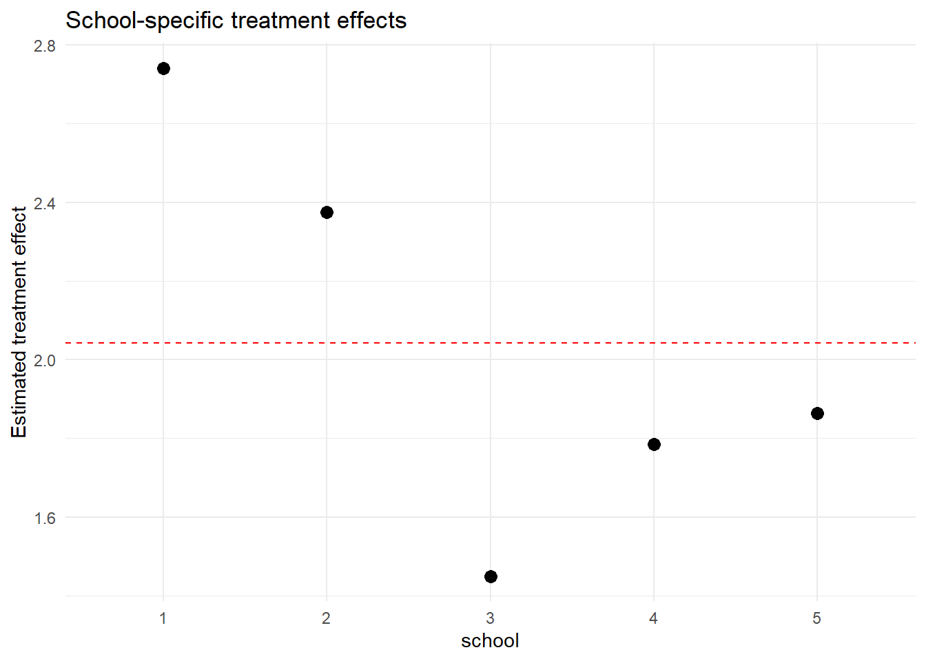

The dashed red line shows the average treatment effect, while the points show each school’s deviation.

1.5 Predicted Lines per School

df_nested$pred <- predict(m_nested)

ggplot(df_nested, aes(x = treatment, y = y, group = school, color = school)) +
  stat_summary(fun = mean, geom = "point", size = 3, position = position_dodge(0.3)) +
  stat_summary(fun = mean, geom = "line", aes(group = school), size = 1) +
  labs(y = "Outcome", title = "Varying treatment effects by school") +
  theme_minimal()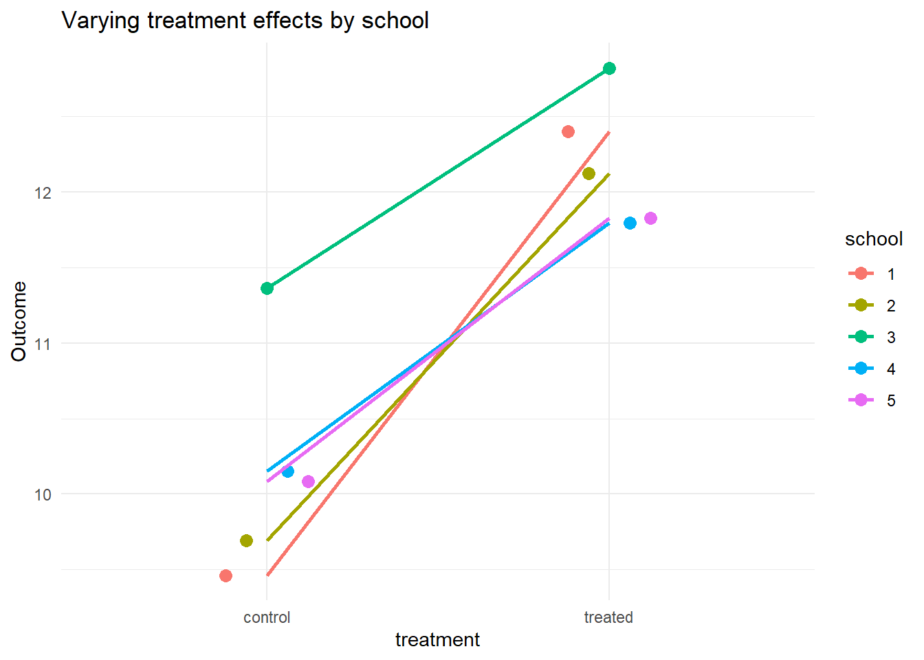

Each line shows how a school responds differently to treatment — some respond more strongly, some less.

1.6 Correlation Between Random Intercepts and Slopes

vc <- VarCorr(m_nested)
vc

##  Groups   Name             Std.Dev. Corr  
##  school   (Intercept)      0.70996        
##           treatmenttreated 0.56111  -0.842
##  Residual                  0.95155

attr(vc$school, "correlation")[1, 2]

## [1] -0.8417701

This value shows how much the intercepts and slopes co-vary. A positive number means that schools with higher baselines tend to have stronger treatment effects, and vice versa. Here, we have a strong negative correlation, meaning that schools with lower baselines will have stronger treatment effects.

Workflow 2: Crossed Random Effects (Students × Raters)

Now we simulate a crossed structure, specifying that each student is rated by multiple raters. Just like we’ve done, we will:

Simulate a dataset where each student can be rated by multiple raters.
We will maintain the two hypothetical treatments namely control and treated.
Remeber, control and treated can be interpreted as two distinct sets of students (e.g., male vs female; undergraduate vs graduate, etc)

2.1 Data Generation for Crossed Model

set.seed(123)
n_students <- 40
n_raters <- 6

df_crossed <- expand.grid(
  student = factor(1:n_students),
  rater = factor(1:n_raters),
  treatment = factor(c("control","treated"))
)

rater_intercepts <- rnorm(n_raters, 0, 2)
rater_slopes <- rnorm(n_raters, 3, 0.7)

df_crossed$score <- 50 +
  rater_intercepts[as.numeric(df_crossed$rater)] +
  rater_slopes[as.numeric(df_crossed$rater)] * (df_crossed$treatment == "treated") +
  rnorm(nrow(df_crossed), 0, 2)

head(df_crossed)

##   student rater treatment    score
## 1       1     1   control 49.68059
## 2       2     1   control 49.10041
## 3       3     1   control 47.76737
## 4       4     1   control 52.45287
## 5       5     1   control 49.87475
## 6       6     1   control 44.94581

str(df_crossed)

## 'data.frame':    480 obs. of  4 variables:
##  $ student  : Factor w/ 40 levels "1","2","3","4",..: 1 2 3 4 5 6 7 8 9 10 ...
##  $ rater    : Factor w/ 6 levels "1","2","3","4",..: 1 1 1 1 1 1 1 1 1 1 ...
##  $ treatment: Factor w/ 2 levels "control","treated": 1 1 1 1 1 1 1 1 1 1 ...
##  $ score    : num  49.7 49.1 47.8 52.5 49.9 ...
##  - attr(*, "out.attrs")=List of 2
##   ..$ dim     : Named int [1:3] 40 6 2
##   .. ..- attr(*, "names")= chr [1:3] "student" "rater" "treatment"
##   ..$ dimnames:List of 3
##   .. ..$ student  : chr [1:40] "student=1" "student=2" "student=3" "student=4" ...
##   .. ..$ rater    : chr [1:6] "rater=1" "rater=2" "rater=3" "rater=4" ...
##   .. ..$ treatment: chr [1:2] "treatment=control" "treatment=treated"

score = Response variable

treatment = Predictor variable as before

student = Grouping variable A

rater = Grouping variable B

2.2 Fitting the Crossed Model

We will specify tw independent grouping factors, necessitate a crossed model structure

m_crossed <- lmer(score ~ treatment + (1 + treatment | rater) + (1 | student), data = df_crossed)
summary(m_crossed)

## Linear mixed model fit by REML ['lmerMod']
## Formula: score ~ treatment + (1 + treatment | rater) + (1 | student)
##    Data: df_crossed
## 
## REML criterion at convergence: 2035.6
## 
## Scaled residuals: 
##     Min      1Q  Median      3Q     Max 
## -2.9650 -0.6181 -0.0653  0.6521  3.3913 
## 
## Random effects:
##  Groups   Name             Variance Std.Dev. Corr
##  student  (Intercept)      0.02136  0.1462       
##  rater    (Intercept)      3.09372  1.7589       
##           treatmenttreated 0.48899  0.6993   0.28
##  Residual                  3.80187  1.9498       
## Number of obs: 480, groups:  student, 40; rater, 6
## 
## Fixed effects:
##                  Estimate Std. Error t value
## (Intercept)       50.8492     0.7294  69.716
## treatmenttreated   3.1800     0.3364   9.453
## 
## Correlation of Fixed Effects:
##             (Intr)
## tretmnttrtd 0.167

Interpretation

Random intercepts/slopes for raters mean each rater interprets the treatment differently.
Random intercept for students adjusts for repeated measures per student.

2.3 Extracting Rater Effects

fix <- fixef(m_crossed)
ranefs <- ranef(m_crossed)$rater

rater_effects <- data.frame(
  rater = rownames(ranefs),
  intercept = fix["(Intercept)"] + ranefs[,"(Intercept)"],
  treatment_effect = fix["treatmenttreated"] + ranefs[,"treatmenttreated"]
)

rater_effects

##   rater intercept treatment_effect
## 1     1  49.03759         3.503371
## 2     2  49.64948         2.447363
## 3     3  52.77535         2.944621
## 4     4  49.94620         2.614150
## 5     5  50.45341         3.621322
## 6     6  53.23342         3.949471

2.4 Visualizing Rater Treatment Effects

ggplot(rater_effects, aes(x = rater, y = treatment_effect)) +
  geom_point(size = 3) +
  geom_hline(yintercept = fix["treatmenttreated"], linetype = "dashed", color = "red") +
  labs(y = "Estimated treatment effect", title = "Rater-specific treatment effects") +
  theme_minimal()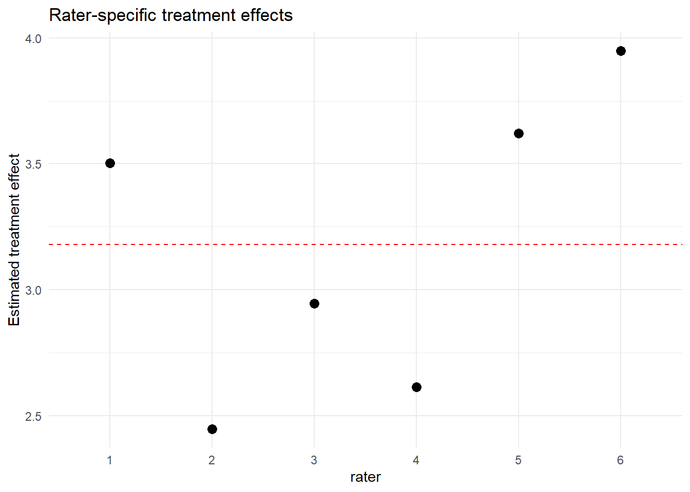

2.5 Predicted Scores by Rater

df_crossed$pred <- predict(m_crossed)

ggplot(df_crossed, aes(x = treatment, y = pred, group = rater, color = rater)) +
  stat_summary(fun = mean, geom = "point", size = 3, position = position_dodge(0.3)) +
  stat_summary(fun = mean, geom = "line", aes(group = rater), size = 1) +
  labs(y = "Predicted score", title = "Varying treatment effects by rater") +
  theme_minimal()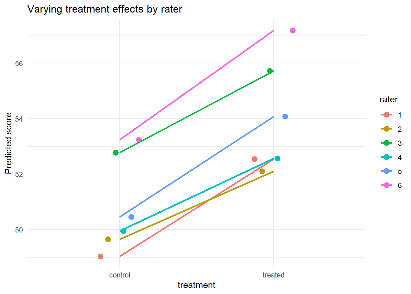

Each rater interprets “treatment” differently, leading to variability in slopes.

2.6 Random Effect Correlation

VarCorr(m_crossed)

##  Groups   Name             Std.Dev. Corr 
##  student  (Intercept)      0.14617       
##  rater    (Intercept)      1.75890       
##           treatmenttreated 0.69928  0.277
##  Residual                  1.94984

The covariance section again shows how intercepts and slopes for raters co-vary.Here, there is a weak positive correlation, meaning that raters with higher baselines have stronger treatment effects.

Summary

Let’s do a quick recap:

Random intercepts capture baseline variability across groups.
Random slopes capture variability in the effect of a predictor across groups.
Correlation between intercepts and slopes tells whether groups with higher baselines show stronger or weaker responses.
Mixed models balance flexibility (allowing variation) with efficiency (borrowing strength across groups).

Hands-On Exercise

Let’s do a quick class work to demonstrate what we have learnt so far. Here, we are going to use a real dataset present in the lme4 package.

Objective:

Fit and interpret a mixed-effects model with random slopes and intercepts using a new dataset.

Dataset:

Use the built-in sleepstudy dataset in lme4. Run ?sleepstudy to understand that dataset.

data("sleepstudy")
head(sleepstudy)

##   Reaction Days Subject
## 1 249.5600    0     308
## 2 258.7047    1     308
## 3 250.8006    2     308
## 4 321.4398    3     308
## 5 356.8519    4     308
## 6 414.6901    5     308

Tasks:

Fit a model predicting Reaction as a function of Days with random intercepts and slopes for Subject:

m_exercise <- lmer(Reaction ~ Days + (1 + Days | Subject), data = sleepstudy)
summary(m_exercise)

Interpret:
- What do the fixed effects mean?
- How do random intercepts and slopes vary across subjects?
- What does the correlation between them imply?
Plot subject-specific slopes using:
```
coef(m_exercise)$Subject
```
Discuss:
- Why do some subjects show stronger or weaker effects of Days on Reaction?
- What happens if we remove the random slope term?

Understanding Random Intercepts and Slopes in Mixed-Effects Models using lme4 and glmmTMB

Grecia, Joshua and Lawrence

11-04-2025

Background

Why multi-levels matter

Fixed vs Random Effects

Nested vs Crossed Random Effects

Benefits of multi-level models

When to use which?

We will focus on `lmer` to explain random slopes and intercepts

Random Intercepts and Random Slopes

Syntax in `lme4`

Correlation Between Intercepts and Slopes

Let us work through examples for nested and crossed random effects

Workflow 1: Nested Random Effects (Schools and Students)

1.1 Data Generation for Nested Model

1.2 Fitting the Nested Model

Interpretation

1.3 Extracting Random Effects

1.4 Visualizing Random Slopes

1.5 Predicted Lines per School

1.6 Correlation Between Random Intercepts and Slopes

Workflow 2: Crossed Random Effects (Students × Raters)

2.1 Data Generation for Crossed Model

2.2 Fitting the Crossed Model

Interpretation

2.3 Extracting Rater Effects

2.4 Visualizing Rater Treatment Effects

2.5 Predicted Scores by Rater

2.6 Random Effect Correlation

Summary

Hands-On Exercise

Objective:

Dataset:

Tasks:

Understanding Random Intercepts and Slopes in Mixed-Effects Models using lme4 and glmmTMB

Grecia, Joshua and Lawrence

11-04-2025

Background

Why multi-levels matter

Fixed vs Random Effects

Nested vs Crossed Random Effects

Benefits of multi-level models

When to use which?

We will focus on lmer to explain random slopes and intercepts

Random Intercepts and Random Slopes

Syntax in lme4

Correlation Between Intercepts and Slopes

Let us work through examples for nested and crossed random effects

Workflow 1: Nested Random Effects (Schools and Students)

1.1 Data Generation for Nested Model

1.2 Fitting the Nested Model

Interpretation

1.3 Extracting Random Effects

1.4 Visualizing Random Slopes

1.5 Predicted Lines per School

1.6 Correlation Between Random Intercepts and Slopes

Workflow 2: Crossed Random Effects (Students × Raters)

2.1 Data Generation for Crossed Model

2.2 Fitting the Crossed Model

Interpretation

2.3 Extracting Rater Effects

2.4 Visualizing Rater Treatment Effects

2.5 Predicted Scores by Rater

2.6 Random Effect Correlation

Summary

Hands-On Exercise

Objective:

Dataset:

Tasks:

We will focus on `lmer` to explain random slopes and intercepts

Syntax in `lme4`