Lab 3: Age-structured populations
NRES 470/670
Spring 2026
In this lab we will have an opportunity to build more complex population models in InsightMaker. Among the concepts we will play around with are age structure, life tables, and simulating the dynamics of age-structured populations.
Mathematics of age-structured populations
Life tables
Let’s start with some definitions- population ecology is full of terms and equations. We should be aware of the meaning of the major terms involved in life table analysis!
Cohort: A collection of organisms born in a population at the same time (i.e., during the same year or breeding season)
x: Age, or time since the birth of the cohort (usually in units of years).
S(x): Total survivors, or census size – the number of individuals in the cohort that survived to age x.
D(x): Total deaths – the number of age-x individuals in the cohort that died before reaching age x+1 (i.e., that died sometime in the interval between x and x+1)
Birth rate, b(x): Average number of offspring produced by individuals in age x (per-capita birth rate for individuals of age x).
Survivorship, l(x):
\[l(x) = \frac{S_x}{S_0} \qquad \text{(Eq. 1)}\] ,where \(S_x\) is the number of survivors from the original cohort at year \(x\). Survivorship represents the fraction of the cohort that is expected to survive to a given age.
Survival rate, g(x):
\[g(x) = \frac{S_{x+1}}{S_x} \qquad
\text{(Eq. 2)}\]
,where \(S_x\) is the number of survivors from the original cohort at year \(x\) (per-capita survival rate at age x). Survival rate is the fraction of individuals in the cohort that survive from age x to age x+1. Another way of thinking of this is as the survival rate for age x individuals conditional on having survived to age x.
Maximum lifespan, k: the age after which all members of the cohort have died.
Lifetime reproductive potential:
\[R_0 = \sum_{x=0}^k l(x)\cdot b(x) \qquad
\text{(Eq. 3)}\]
Lifetime reproductive potential is the average number of female offspring produced per female over her entire lifetime.
Life Expectancy (for a newborn) can be approximated as:
\[LE_0 = \frac{\sum_{x=0}^{k}S(x+1)+0.5*D(x)}{S(0)} \qquad \text{(Eq. 4)}\]
Q: why is the above estimate for life expectancy (LE) approximate and not exact?
Generation time is defined as the Average age of individuals in the cohort when they produce offspring (for all offspring born to the cohort, record the age of the mom at the time she gave birth, and then take the average of all these ages!). This can be computed as:
\[G = \frac{\sum_{x=0}^{k}l(x)\cdot b(x)\cdot x}{\sum_{x=0}^{k}l(x)\cdot b(x)} \qquad \text{(Eq. 5)}\]
Intrinsic rate of growth, \(r\) is defined (approximately) as:
\[r = \frac{ln(R_0)}{G} \qquad \text{(Eq. 6)}\]
lambda, \(\lambda\) is defined (to a first-order approximation) as: \(\lambda = e^{r}\)
NOTE: the Gotelli book describes a more exact way to compute the intrinsic rate of growth from life tables, called the Euler method. You are not required to know how to use the Euler method in this class, but I recommend playing around with it, because it is widely used in population ecology.
One more concept I want to introduce here is reproductive value, or V(x). This represents the expected future reproductive output of an individual of age x, adjusted for the intrinsic rate of growth:
\[V(x) = \frac{e^{rx}}{l(x)}
\sum_{y=x+1}^{k}e^{-ry}l(y)b(y) \qquad \text{(Eq. 7)}\]
Different individuals in a population tend to have different “value” in
terms of contributing to future generations. Caswell (2001) said “The
amount of future reproduction, the probability of surviving to realize
it, and the time required for the offspring to be produced all enter
into the reproductive value of an age-class”. Knowing something about
the relative “value” of different individuals in a population can help
managers decide which individuals to translocate, or to harvest, or cull
from a population. Therefore, Reproductive Value is critical for applied
population ecology! Reproductive Value also factors heavily in
evolutionary studies and life history theory.
Generally, reproductive value is maximized around the age of first reproduction. This concept is also very important in evolutionary biology, since alleles that affect individuals of high reproductive value are likely to be more heavily influenced by natural selection. Conversely, deleterious alleles that affect elderly individuals are not necessarily going to be swept from a population- one possible explanation for senescence!
Q: Why is the reproductive value adjusted by the population growth rate??
Here is a sample life table for practice!! click here to download
And here is a more complex life table- for even more practice! This one is based on Peter and Rosemary Grant’s work with the Galapagos finches. This life table is based on their data for cactus finches! click here to download. You probably want to convert it to Excel format before working with it.
Exercise 1: life table analysis
Let’s imagine that we are following a cohort of reintroduced Chatham Island robins on a small island through time.
- First, we establish artificial nests and place 400 captive-laid eggs
in them.
- All individuals are given a unique marking as soon as they hatch
(hatching is 100% successful!). These markings are permanent and not
affected by tag loss!
- We visit the island once per year, and count all the female
individuals with tags who still exist in the population. We can assume
that if the individual is alive then we will observe it (perfect
detection!). If we do not see the individual we know with certainty that
it is dead!
- Of the original robins released on the island, we record the following numbers over 5 years revisiting the island (starting with 400 at year 0): 175 (year 1), 103 (year 2), 45 (year 3), 19 (year 4), and 0 (year 5).
- We record the following per-capita reproductive rates for each age: 0, 0.8, 2.4, 2.9, 0.4, and 0
You can load these data in this file. It should look something like this:
| x | S(x) | b(x) |
|---|---|---|
| 0 | 400 | 0.0 |
| 1 | 175 | 0.8 |
| 2 | 103 | 2.4 |
| 3 | 45 | 2.9 |
| 4 | 19 | 0.4 |
| 5 | 0 | 0.0 |
QUESTIONS, Exercise 1 (black robin example):
First, plot the survivorship curve. Specifically, make a new plot in Excel with survivorship on the y axis and age on the x axis. Make sure to display survivorship on the logarithmic scale. One way to do this is to make a scatterplot of raw survivorship (l(x)) against age, then double-click on the y-axis and choose the “logarithmic scale” option. Alternatively, you can make a new column representing the log of survivorship (you can use log base 10 or natural log) and plot that new variable (log l(x)) as a function of age. Either way, don’t plot the final year- since the log of zero is not defined!
NOTE: Please refer to the ‘age-structured populations’ lecture page for more information on survivorship curves.
1a (image upload). Upload your plotted survivorship curve (log survivorship vs age, see above) for the black robin. Make sure your axes are properly labeled.
1b (short answer). Based on the survivorship curve you made for the black robin (plot from 1a, above), does this population most closely resemble type I, II, or III survivorship? Briefly explain your reasoning.
1c (numeric input and short answer). What is the lifetime reproductive potential, \(R_0\) for this population? Based on your estimate of \(R_0\) (1c, above) is this population growing, declining or stable?
1d (numeric input). What is the estimated life expectancy at birth, \(LE\), for this black robin population?
1e (numeric input). What is the estimated generation time, \(G\) for this black robin population, in years?
1f (numeric inputs and short answer). What is the reproductive value(\(V\)) for each age (x) in this population? Which age is associated with the highest reproductive value?
ASIDE: If you wanted to start a new population of black robins on a different island, you might choose to translocate individuals at this age to maximize the probability of success with the fewest number of translocatees!
For the following questions (1g and 1h), set the value of b(1) (cell C3 in Excel) to zero. When you do this, you are effectively delaying the age at reproduction by one year.
1g (numeric input and short answer). After making this change (i.e., delay age-at-maturity by one year), what is the new lifetime reproductive potential, \(R_0\) for this population? Based on your new estimate of \(R_0\), is this population growing, declining or stable?
1h (numeric input). After making this change (i.e., delay age-at-maturity by one year), what is your new estimate for the generation time \(G\) for this population, in years?
1i (written response). Imagine you have the following population of black robins this year: 100 individuals of age 0 (newborns) and 10 individuals of age 1. No older indviduals (age 2, 3, 4) exist on the island at this time. How many newborn robins (age 0) would you expect to be born one year from now, assuming no new robins will be born in the population until right before you survey the population next year? Explain how you got your answer!
NOTE: you do not need to use InsightMaker or Excel here (although you could!)- just think it through and use a calculator if needed
HINT: the age 0 individuals will be 1 years old next year, and the 1-year-olds this year will be two years old next year
HINT: in order to produce offspring one year from now, individuals must first survive to next year!
Exercise 2: another life table analysis

Let’s take the Uinta ground squirrel example from the Gotelli book. Take a minute to read the description in Gotelli (end of Ch. 3)…
This is real data set from a long-term experimental study. However, the version you see below is modified from the Gotelli book so it’s easier to work with!
The first life table (on the left) represents a cohort of ground squirrels in a population at typical densities.
The second life table (right) represents a cohort of ground squirrels in a population at lower-than-average densities (many individuals were removed from the population prior to the start of the experiment).
Load up the Uinta ground squirrel life table data given to us by Gotelli (reproduced from Slade and Balph 1974 – and modified slightly to make it easier to work with).
QUESTIONS, Exercise 2: Uinta ground squirrel example
For the following questions (2a and 2b), Compare the two life tables (pre-density reduction vs post-density reduction).
2a (Numeric inputs and short answer). What is the lifetime reproductive potential (\(R0\)) and intrinsic rate of growth (\(r\)) for the Uinta ground squirrels, both before and after the density reduction experiment? Based on this result, write one sentence explaining whether population growth rate was faster or slower after the density-reduction experiment.
2b (short answer). If the change in population growth rate you reported in 2a was driven by a density-dependence mechanism (e.g., competition for resources, safety in numbers), would you consider this study as an example of negative density dependence (a stabilizing force potentially resulting in population regulation) or positive density dependence (also known as an Allee effect - which can be a destabilizing force that can induce rapid extinction)? Explain your reasoning.
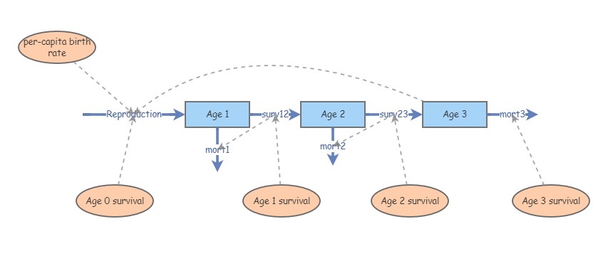
Exercise 3: age-structured models in InsightMaker
Let’s first build an age-structured model from scratch in InsightMaker. To do this, you can follow these steps:
Open a blank workspace and save it.
Make three new stocks in your canvas: Age 1, Age 2 and Age 3. The Age 1 stock represents individuals that have lived for full year - we can think of these individuals has just about to celebrate their first birthday! Since the model runs on a one-year time step, these individuals all transition to the Age 2 stock if they survive. The surviving Age 2 individuals transition to Age 3. In this model, we assume that all individuals in this population die before they reach age 4.
Make a new flow ([Flow In]) called Reproduction. This should represent new Age 1 individuals added to the population each year. We will ignore immigration, so new additions into the Age 1 stock are the only way to add new individuals into this population. We will assume that individuals are capable of reproduction at exactly 3 years of age. This species is semelparous- that is, it can only breed once in its lifetime! Therefore, draw [Links] from Age 0 and Age 1 to Reproduction.
But wait, where are the newborns (Age 0 individuals)???
In this model, we assume that this population has a breeding pulse once per year, and that we survey the population right before the birth pulse each year. Therefore, we can’t keep track of the number of newborns (Age 0 individuals) in the population because we can’t observe them. All we can observe are the new one-year-olds in the population- these are the individuals that were born right after our last survey (and who are now nearly one year of age). This is known as a pre-breeding census model. One consequence of this is that the Reproduction flow in this model should only represent those individuals that were born last year and survived to this year!
NOTE: this is one of the trickier concepts in population ecology. We will revisit this in more detail in Lab 4 (matrix population models).
Make new flows from Age 1 to Age 2 and from Age 2 to Age 3, called Transition to Age 2 and Transition to Age 3, respectively (yes, you can use Flows to connect two Stocks!). These flows represent the number of individuals from Age 1 that move into the Age 2 stock, and from Age 2 to Age 3. Another way to think of these flows is that they represent the number of survivors from one stage to the next! When you are making these flows from one [Stock] to another, drag the [Flow] out from the arrow on the first stock, and keep dragging until the second stock is highlighted on the canvas- that way you can be sure the two stocks are connected!
Make three new [Flows Out] representing mortality, emerging respectively from each stock and called Age 1 mortality, Age 2 mortality, and Age 3 mortality.
Make a new variable called Age 3 birth rate representing the per-capita birth rate for individuals that are exactly 3 years of age. Make another variable called Age 0 survival, representing the survival rate from newborn (age 0) to age 1. Draw links from these variables to the Reproduction flow. Also, draw links connecting the Age 0 survival and Age 3 birth rate variables to the Reproduction flow.
Make three new variables representing the per-capita survival rates from one stage to another, called Age 1 survival, Age 2 survival, and Age 3 survival. Draw links to the appropriate flows. NOTE: these transition rates are also sometimes called “growth rates” in population ecology.
Draw links from the survival flows going out of a particular stage (e.g., Transition to Age 2) to the mortality flow out of the same stage (e.g., Age 1 mortality). This way, you can define total mortality as the number of individuals in the stage (in the stock) minus the number of survivors (everyone who doesn’t survive must die). In the mortality flows, this will look something like this:
[Age 1]-[Transition to Age 2]- Make a new variable called TotN, representing total abundance. Make “Ghost primitives” for each of the three stocks, and move the “ghosts” next to the TotN variable. Draw links from each ghost stock to the TotN variable. In the equation editor for TotN, compute the sum of the 3 stocks. You may want to group these together into a folder to keep your canvas tidy.
Your new insight should look something like this:
- Parameterize your new age-structured population!
Age 3 birth rate: 12 (12 female offspring per female, assuming a female only model) Age 0 survival: 0.1 (10%) Age 1 survival: 0.9 (90%) Age 2 survival: 0.5 (50%) Age 3 survival: 0 (100% mortality- no individuals survive to age 4) Initial N, Age 1: 100 Initial N, Age 2: 100 Initial N, Age 3: 50
For each of the remaining [Flows] in the model, use the equation editor to specify the appropriate equations. First click on the equation editors for the survival flows (e.g., transition from age 1 to 2), and specify the appropriate equations. Finally, click on the Reproduction flow, and specify the appropriate equation.
Explore the model- make sure you understand how it works!
I encourage you to build your own age-structured IM model, but I will also provide a link to a “skeleton” version of the model so you can focus on the concepts and not struggle too much with the modeling. Here is the “skeleton” version (all the structure but none of the parameters or equations) of the model: https://insightmaker.com/insight/2AdLJcyceguszkSt3EK89/Age-structure-lab-3-skeleton
QUESTIONS, Exercise 3 (age-structured model in InsightMaker):
3a (equation and short answer). What is your equation for Reproduction flow in the above model (flow into the Age 1 stock)? Copy and paste your equation from InsightMaker. Using plain English, explain why this is the correct equation for computing the number of age 1 individuals entering the population each year.
3b (image upload). Initialize the population abundances (initial abundances for Age 1, Age 2, and Age 3) so that your population consists of only 100 individuals in the first age class (i.e., 100 individuals in Age 1, no individuals in the other age classes). Run the model for 30 years in Insightmaker, and upload the resulting plot of abundance over time as an image file.
NOTE: this should be a declining population!
3c (numeric input and short answer). Imagine you could enact a predator-control program and increase the survival of Age 0 individuals (first-year survival rate). What is the smallest value of first-year survival (survival from newborn to age 1) that would cause this population to grow over time (keeping all other parameters at the values stated above)? Briefly explain how you got your answer.
3d (InsightMaker URL. Please share the URL for your Insight: save your model as a ‘Public Insight’ and insert the URL into WebCampus in the appropriate place. And don’t make any more changes to this insight once you have submitted it (use a cloned version if you want to keep making changes)!
Checklist for Lab 3 completion
Please type your responses into one Word document and submit using WebCampus! See submission deadline on WebCampus.
- Exercise 1
- Image upload (1a.)
- Short answer (1b.)
- Short answer (1c.)
- Short answer (1d.)
- Short answer (1e.)
- Short answer (1f.)
- Short answer (1g.)
- Short answer (1h.)
- Short answer (1i.)
- Image upload (1a.)
- Exercise 2
- Short answer (2a.)
- Short answer (2b.)
- Exercise 3
- Short answer (3a.)
- Image upload (3b.)
- Short answer (3c.)
- InsightMaker URL (3d.)
- Exercise 1
Completely optional: exercise 4: more complex age-structured models in InsightMaker!
Implement the following density-dependent model (modifying your previous age-structured model in InsightMaker). If the total population (all three age classes combined!) exceeds 75 individuals, then birth rate drops to 25% of normal rates (declines by 75%).
4a (optional). Change the Age 0 survival rate to 0.75 (from 0.1). Run the simulation starting with initial abundances as described earlier (100, 100, and 50). Describe the resulting population dynamics. Is this a random (stochastic) model (different results every time you run the model, even with the same initial conditions)? Explain your reasoning.