Metapopulations
NRES 470/670
Spring 2026
Upcoming midterm exam
when and where The second midterm exam (out of two) is coming up on Wednesday April 22. You will have the whole class period to take the exam. We will use the same basic format as we used for the first midterm.
what The exam will cover:
- All material in Chapters 1-4 of the Gotelli book:
- Chapter 1: Exponential growth
- Chapter 2: Logistic growth
- Chapter 3: Age structured population and matrix models
- Chapter 4: Metapopulations
- All material covered in lectures, including the following web pages:
- Systems thinking and modeling
- Exponential growth
- Malthus and limits to growth
- Logistic population growth
- Allee effect
- Age-structured populations
- Matrix population models
- “Embracing” uncertainty (this and below are new topics for this exam)
- Small-population paradigm
- Declining-population paradigm
- Population Viability Analysis (just the part at the top, before the section called “The PVA Process”- the rest is there to help with final projects)
- Metapopulations and source-sink dynamics
- NOTE: all lectures have been recorded and are available via the
“Zoom” link on WebCampus in case you missed any or in case you’d like to
use these recordings as review/study materials
- All material covered in labs 1-6, including:
- Basic programming concepts:
- Conditional logic (IF-THEN-ELSE): see examples in Malthus and Allee effect lectures
- Iteration (‘FOR loops’): see examples in Lab 1 and Lab 4.
- NOTE: you will NOT be tested on how to run population models in R (or how to do anything else in R).
The exam will consist of a mixture of multiple-choice and short-answer questions.
We will do a review session in class on Monday April 20. Please make note of any questions that come up as you study- we can talk these over during the review session!
Metapopulations
What is a metapopulation?
Broadly speaking, a metapopulation is a group of populations (often called subpopulations) that occupy spatially distinct habitat patches and where some movement of individuals among patches is possible.
Now that we’re thinking about animals occupying habitat patches within a larger landscape, we need to incorporate information about movement ecology (and spatial ecology) in addition to population ecology!
Patches in a metapopulation are connected via dispersal of individuals among patches (also known as connectivity).
In practice, metapopulation ecology covers a broad range of scenarios: as long as we can conceive of subpopulations occupying distinct habitat patches in a landscape, then we can model this set of populations through the lens of metapopulation ecology.
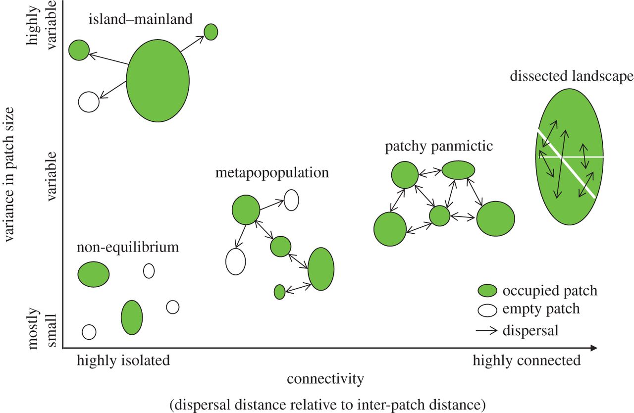
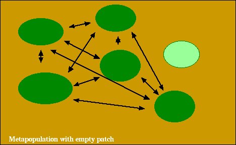
NOTE: in some definitions, a “metapopulation” is more narrowly defined as a set of similar patches with limited connectivity and with at least some unoccupied patches at each time period (see figure below). I prefer the more inclusive definition!
The term “classical metapopulation model” refers to models where we don’t keep track of abundance (\(N\) is no longer our primary unit of interest). Instead, we only consider patch occupancy (the number or fraction of patches in the metapopulation that are occupied) - like the models in Gotelli Chapter 4.
That is, we only care about whether a patch is occupied (\(N > 0\) in a given patch) or not (\(N = 0\)) each year.
In ‘classical’ metapopulation models, we assume that all areas outside a patch are completely unsuitable (i.e., they are NOT habitat, although individuals may be able to move between patches via dispersal).

However, we CAN keep track of patch abundance in a metapopulation model if we really want to (like the more complex metapopulation model in the final part of lab 6!).
The simplest classical metapopulation models (like those in Gotelli Ch 4) don’t even keep track of the number of occupied patches on the landscape- they only keep track of the fraction of occupied patches in the landscape (\(f\))!
Instead of keeping track of the number of individuals dispersing among patches, classical metapopulation models only consider the consequences of dispersal, which include colonization of unoccupied (empty) patches and the rescue effect (immigration preventing extinction of a patch; see below).
“Classical” metapopulation models
The metapopulation concept was first introduced by ecologist Richard Levins in 1969, and further developed by Ilkka Hanski among others.
In a classical metapopulation, the [Stock] we are studying now is NOT the total number of individuals but instead it is the fraction of patches occupied, \(f\)!
Instead of investigating population dynamics, we are investigating metapopulation occupancy dynamics – that is, how the fraction of occupied patches changes over time (\(\Delta f\).
How does a metapopulation grow? How does a metapopulation shrink?
colonization is the process of a patch transitioning from unoccupied to occupied via immigration from an external source!
extirpation (or extinction) is the process of a patch transitioning from occupied to unoccupied.
More formally, here are some terms we will consider:
\(f_t\) is the fraction, or
proportion, of patches that are occupied at time \(t\). This is also known as the
fractional occupancy. This is the primary [Stock] we
model in a classical metapopulation model.
\(I\) is the total fraction of patches
that are colonized (by immigrants) per time period (colonization
rate).
\(E\) is the total fraction of patches that are extirpated per time period (extirpation rate).
Therefore, the change in occupancy \(\Delta f\) can be expressed as:
\(\Delta f = I - E\)
\(p_i\) is the probability of colonization for any non-occupied patch.
\(p_e\) is the probability of extinction for any occupied patch.
Now that we have the basic terms defined, we can build a basic model of metapopulation dynamics! We will do this in lab 6- refer to the metapopulation lab for more details!
Assumptions of the classical metapopulation model:
Classical metapopulation models assume:
- Homogeneous patches (all patches are considered equal and
interchangeable- they do not differ in size or quality – any differences
in habitat quality or spatial context within patches are ignored). We
will relax this assumption when we start to consider ‘source and sink’
models (below).
- Extinction and colonization are insensitive to spatial context
(spatial context, or “neighborhood effects”, do not affect \(p_e\) and \(p_i\)).
- No time lags (metapopulation growth responds instantaneously to any
changes in \(f\)).
- Very large number of patches (even when the fraction of occupied patches \(f\) is very small, the classical metapopulation still persists!). That is, global extinction is not possible!
Clearly this is not a very realistic model, but it is a useful starting place. So.. we will start by making these assumptions, but then we will “relax” some of them!
Variant #1: island-mainland model
Colonization occurs via immigration from a constant external source – a constant propagule rain.
This is the simplest metapopulation model. \(p_i\) and \(p_e\) are constant.
Variant #2: internal colonization
Now, colonization can only happen via immigration from within the metapopulation itself. So when a small fraction of patches are colonized, the colonization probability is low because of a lack of potential immigrants within the metapopulation.
\(p_i = i\cdot f\)
\(i\) represents the strength of internal immigration (how much the probability of colonization increases with each new occupied patch in the metapopulation.
In this model, the colonization rate approaches \(i\) as nearly all patches become occupied, and approaches zero as the metapopulation approaches global extinction
Variant #3: rescue effect.
Now, the extinction rate can be reduced by immigration from other populations in the metapopulation!
Q: does this make sense? How does the rescue effect work?
\(p_e = e(1-f)\)
In this model, the extinction rate approaches 0 as the metapopulation approaches full occupancy [note, this may not be realistic, as it implies a perfectly successful rescue effect!].
On the other hand, the extinction rate approaches \(e\) as the metapopulation approaches global extirpation (when there are little to no immigrants from other occupied patches that could ‘rescue’ an occupied patch from extinction).
‘Dynamic’ stability
In the classical metapopulation model, extinction is not necessarily uncommon. Patches go extinct – small patches can be highly vulnerable to demographic stochasiticity as we know! – but as long as patches can get re-colonized, we can reach an equilibrium, where extinctions and colonizations cancel each other out. In a classical metapopulation model, this is often a stable equilibrium, and a stable metapopulation in which local extinctions are possible (\(p_e > 0\)) is called dynamically stable. That is, any given patch could be extinct at any given time, but on the whole, the size of the metapopulation (total patches occupied) is relatively stable and not at risk of regional (or global) extinction!
The concept of dynamic metapopulation stability- in which extinctions and colonizations balance out - has much in common with the dynamic stability of a single population at carrying capacity - in which any given individual could die at any given time, but deaths and births approximately balance out!
Global extinction
global extinction represents extinction (extirpation) of all patches in the metapopulation.
Q: what is the analog of demographic stochasticity in a metapopulation model? [Top Hat]
NOTE: the “individual” in a metapopulation model is a patch. The analogy to “death” in a metapopulation is extinction.
Spreading the risk!
In the classical metapopulation models, we assumed there were a very large number of patches in our landscape, so there was no real chance of regional/global extinction. But most real metapopulations are small enough such that we often need to consider the risk of global extinction.
Let’s consider a system in which a species occupies a single patch, and there is a probability of extinction \(p_e\) of 0.15 per patch per year.
Q: What is the probability of regional extinction over the next 10 years?
The probability of persistence for 1 year is \(1-p_e\), so the probability of persistence for 10 years is \((1-p_e)^{10}\) and the probability of regional extinction is \(1-((1-p_e)^{10})\)
which works out to be about 80%. There is a substantial probability of regional extinction sometime over the next 10 years!
What if there were two patches instead of just one?
Let’s assume that the extinction risk for the two patches are independent – that is, the extinction of one patch doesn’t influence whether or not the other patch goes extinct! This is a critical assumption.
If the probability of extinction of one patch over the next 10 years is 0.8, then the probability of both patches going extinct sometime over the next 10 years is 0.8*0.8 = 0.64
So the chance of regional extirpation is somewhat reduced with two populations!!
This is an example of spreading the risk.
What if there are 5 independent populations instead of two? Then what is the chance of regional extirpation over 10 years?
\([1-(1-p_e)^{10}]^5\)
This works out to be around 33%
What if there are 15 independent populations instead of five? Then what is the chance of regional extirpation over 10 years?
\([1-(1-p_e)^{10}]^{15}\)
This works out to be around 4% – we have effectively spread out the risk, so that despite a relatively high extinction risk at the patch level, the metapopulation is unlikely to experience global extinction
Q: if we included dispersal among patches, would dispersal serve to further reduce the risk of global extinction? Why or why not?
By the rescue effect, the risk of extinction may be reduced in this scenario.
However, if the patches are close enough geographically to allow for substantial dispersal, the risk of extinction may be correlated among these two patches!
Q: What if the extinction of one patch was perfectly correlated with the extinction of all other patches? If one patch goes extinct, all go extinct. Specifically, what is the risk of global extinction over a 2-year period, given that the annual risk of extinction is 50% for each patch? [Top Hat]
bonus question: what is the risk of global extinction assuming the risk of extinction in each of the two patches is not correlated (completely independent of one another)?
Sources and sinks!
One important and practically useful concept related to metapopulations is that of source-sink dynamics
In the real world, patches vary in size and quality. That is, the assumption of homogeneity of patches (inherent to the classical metapopulation framework) is unlikely to be met in most real metapopulations!
That is, vital rates and abundances can vary over space. Some areas might have better habitat, with higher overall population growth rates! On the other hand, some areas might have poor habitat- and these areas may be associated with lower vital rates.
In fact, some habitat patches may be so resource-poor or afford ineffective refuge from predators - such that population growth is negative (i.e., \(r\) below zero, or \(\lambda\) less than 1).
Other patches may represent more optimal conditions for rapid population growth (at least if the habitat isn’t too crowded)!
A source population is defined as a patch with a positive intrinsic growth rate (r>0) that contributes more immigrants to nearby patches than it receives back from these neighboring patches. A source population should persist indefinitely, even in isolation.
A sink population is defined as a patch with a negative intrinsic growth rate (r<0). A sink population would go extinct if it were not for the constant input of immigrants from nearby source populations. Sink populations can not persist in isolation.
A pseudo-sink population is defined as a patch with intrinsic rate of growth above zero (r>0) whose abundance is artifically augmented by immigrants from nearby source populations. In isolation (in the absence of immigration from a nearby source population) a pseudo-sink would not go extinct (a true sink would go extinct!), but would settle at a lower equilibrium abundance (i.e., its own carrying capacity). That is, a pseudo-sink maintains an equilibrium abundance above its carrying capacity due to the influx of immigrants from one or more nearby source populations.
One final definition:
If a sink habitat is also very attractive to a species, this can be considered a form of ecological trap (or evolutionary trap). This can happen when human land use practices (to which a species is not evolved) transforms what a focal species perceives as good habitat (following signals that have indicated high-quality habitat over evolutionary time) into a “death trap”. For instance, some birds are evolved to nest in open fields. To these species, hayfields may seem like a good place to nest- but then the mowers and balers come through and destroy all the nests. Such habitat is an especially dangerous type of sink habitat for conservation!!
On the flip side, the ecological traps can be used to help manage pest species. For example, Napier grass (Pennisetum purpureum) is planted as a border around maize fields in east Africa. Stem borer moths (Busseola fusca, Chilo partellus) are strongly attracted to Napier grass for oviposition (they prefer it over maize) but Napier grass produces a sticky substance that physically traps neonate larvae after hatching, killing them before they can establish.
In-class exercise: sources and sinks!
In this exercise, we will explore source-sink dynamics!
- First click on this link and clone this population-based source-sink model in InsightMaker. This model represents a four-patch metapopulation with one large source population and three smaller sink populations. The sink populations are located at varying distances from the source population. Here is the approximate spatial configuration of this metapopulation:
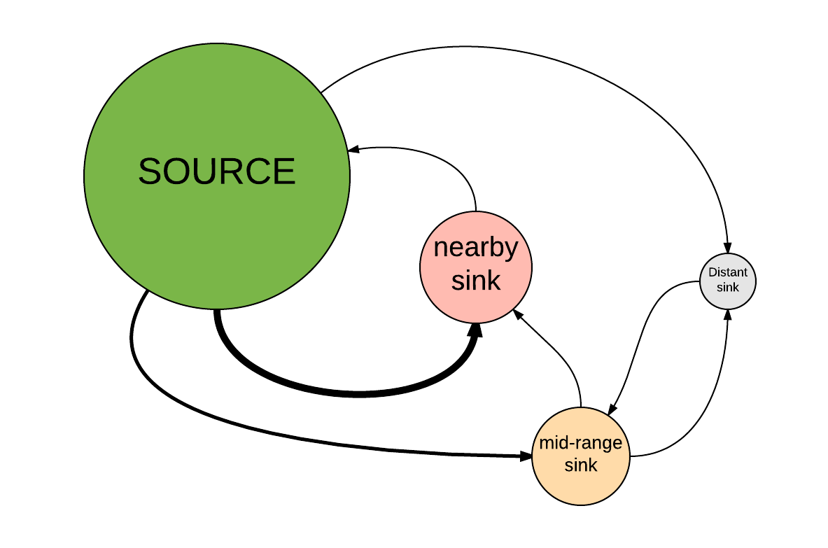
- Make sure the model parameters are at default values. The default parameters should be:
Initial abundance in source: 100
Initial abundance in nearby sink: 10
Initial abundance in mid-range sink: 10
Initial abundance in distant sink: 10
K for source population: 100
K for nearby sink: 50
K for mid-range sink: 25
K for distant sink: 15
Maximum dispersal rate: 10% per year (0.1)
Lambda for source population [lambda good]: 2.1 Lambda (discrete growth
rate) for sink populations [lambda bad]: 0.8
NOTE: maximum dispersal rate (in this model) is the rate of dispersal between neighboring patches. Patches that are located farther apart have dispersal rates that are computed as a fraction of the maximum rate.
Run the model, view the results and make sure you understand how the model works.
Change the dispersal rate to zero and run the model. What happens? Does this make sense?
Change the dispersal rate to 0.01 (1%). What happens now? Does the distant sink still function as a sink population? That is, is it occupied continuously? If not, what is the minimum dispersal rate that generally ensures that the distant sink is continuously occupied (make sure the lower bound of the 95% confidence region for abundance in this patch is above 2 for all years)? [Top Hat]
Now reduce the population growth rate in the source population (“lambda good”) to 1.1. What happens now? Does the source population still operate as an effective source (that is, does it support consistent occupation of all the sinks)?
What happens if you set the maximum growth rate in the source patch to 1? Could such a population ever serve as an effective source population?
A pseudo-sink!
- Change the source lambda back to 2.1. Now change the sink lambda to 1.1 and the max dispersal rate to 25%. What is the approximate equilibrium abundance of the distant sink? How does this relate to its carrying capacity? Generate a figure (using InsightMaker) that illustrates the abundance of the mid-range sink vs. carrying capacity (over time). How does this figure illustrate the concept of a pseudo-sink.
An ecological trap!
- Change all params back to their default values (base scenario). Now consider the following:
NOTE: you may want to clone your model now to enable you to easily go back and forth between the “ecological trap” model and the “source-sink” model.
The nearby sink patch is now extremely attractive to our focal species- since it contains abundant food resources and what seems like good shelter! However, in this habitat there is also a novel, introduced plant that looks like food but is in fact extremely poisonous. Therefore, dispersal rates to the sink habitat are very high, but mortality rates are also very high.
To force a disproportionate number of individuals into the nearby sink, open the equation editor for the flow from the source to the nearby sink. Change the equation to:
0.01*[nearby sink] - 0.5*[SOURCE]NOTE: you can “comment out” what was previously in the equation editor for this flow. To do this, you can either use pound symbols like we have done in the past (and like R!) or we can bracket a whole block of code using the following syntax:
/*
some random
code here
and
some more
random code
*/
This will force 50% of the source population to try to move to the sink habitat each year! Nearly all individuals that are in the sink habitat will attempt to stay there.
Also, change the lambda for the nearby sink to 0.25 (meaning 75% decline each year due to poisoning). To do this, replace the [lambda bad] term in the births/deaths equation for the nearby sink with the number “0.25”. Open the equation editor for this flow- after you change, it should look something like this:
growth <- [nearby sink]*Ln(0.25)

totalexp <- [nearby sink]+growth   # expected population size
newexp <- 0
If totalexp>0.5 Then
  newexp <- RandPoisson(totalexp)
End If
newexp-[nearby sink]
You can clone the ecological trap model here
- Run the model with the nearby sink as an ecological trap, and try to address the following questions:
Q: In what way is the nearby sink now an ecological trap? Are all sink populations really ecological traps?
Q: Are metapopulations better off without sink populations?
Q: Could it ever be desirable to remove a sink population to improve the conservation status of a metapopulation? Under what circumstances?
Benefits of sink populations!
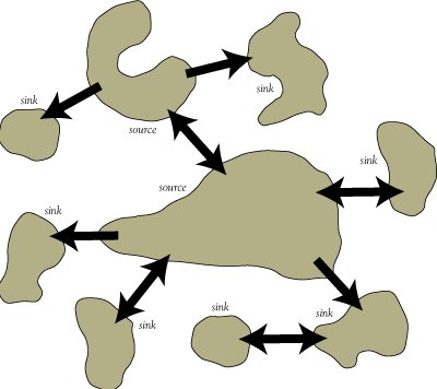
Sink populations may not always be so bad for conservation! Consider the following scenario:
A large source population is able to maintain a set of 3 satellite populations, each of which would not persist in the absence of dispersal from the source population. Occasionally (e.g., once per 100 years), a catastrophic fire eradicates the source population. However, the source population is then colonized by individuals migrating from the satellite (sink) populations. In the absence of the sink populations, the entire metapopulation would almost certainly go extinct!