Lab 4: Matrix population models
NRES 470/670
Spring 2026
In this lab we will continue to work with age-structured populations: specifically, we will get familiar with matrix population models! Remember that while matrix population models may look complicated, they are at their heart a structured version of the discrete exponential growth model: \(N_{t+1}=\lambda \cdot N_t\).
If you want to follow along in R, you can find the R script here. I recommend right-clicking on the link, saving the script to a designated folder, and loading up the script in RStudio.
Mathematics of matrix population models:
We all remember the discrete population growth equation:
\[N_{t+1}=\lambda N_t \qquad \text{(Eq. 1)}\],
where \(N\) represents abundance (as always), \(t\) is time (often in years), and \(\lambda\) is the multiplicative growth rate over the time period \(t \rightarrow t+1\)
In other words, \(\lambda\) is the number you multiply this year’s abundance by to compute next year’s abundance.
The matrix population growth equation looks pretty much the same!
\[\mathbf{N}_{t+1} = \mathbf{A} \mathbf{N}_{t} \qquad \text{(Eq. 2)}\],
where \(\mathbf{N}\) is a vector of abundances (an ordered collection of numbers representing abundances for each life stage), and \(\mathbf{A}\) is the transition matrix (an ordered 2D array of numbers representing per-capita transition rates among life stages from one year to the next).
We can be more explicit about this if we re-write the above equation this way:
\[\begin{bmatrix}N_1\\ N_2\\N_3 \end{bmatrix}_{t+1}=\begin{bmatrix}F_1 & F_2 & F_3\\ P_{1 \rightarrow 2} & P_{2 \rightarrow 2} & 0\\ 0 & P_{2 \rightarrow 3} & P_{3 \rightarrow 3}\end{bmatrix} \cdot \begin{bmatrix}N_1\\ N_2\\N_3 \end{bmatrix}_{t} \qquad \text{(Eq. 3)}\]
Where \(P_{1 \rightarrow 2}\) is the probability of advancing from Stage 1 to Stage 2 (fraction of Stage 1 individuals that survive and transition to Stage 2), and \(F_2\) is the fecundity of stage 2 (per-capita offspring production by individuals that started the year in Stage 2).
The Transition Matrix
The transition matrix must be a square matrix – meaning that the number of rows is the same as the number of columns. There must be the same number of rows and columns as there are life stages for the species you are modeling. If there are 5 life stages, your transition matrix must have five rows and five columns.
Age structured model (Leslie matrix)
The term ‘Leslie Matrix’ refers to a specific type of matrix population model where each stage represents one year of life (this is an age-structured model.
In NRES 470/670, we will always assume that reproduction occurs at the start of each time step. This type of matrix model is known as a “pre-breeding census” because we assume that breeding takes place right after we monitor our population. In this way, the youngest age we ever observe are individuals that were born right after last year’s survey- meaning, nearly one years old! Therefore, we will always assume that the first age class represents one-year-olds (or one month if the model time step is in months or one day if the time step is in days). This is known as a pre-breeding census model - see the Gotelli book for more details. In general, the first row of a transition matrix (i.e., the “fecundity row”) will represent the production of new one-year-olds into the population next year.
Since each cell of a Leslie matrix represents the transition from one age to the next, no individuals can stay the same age for more than one year (obviously). So, terms like \(P_{2 \rightarrow 2}\), or \(P_{3 \rightarrow 3}\) must be set to zero by definition. Each age class is associated with only one survival rate, and this rate involves transitioning to the next age (one year older!). Individuals currently in one age class can only end up in the next age class (assuming they survive). So two year olds can only transition to age 3 (\(P_{2 \rightarrow 3}\)), and three year olds can only transition to age 4 (\(P_{3 \rightarrow 4}\)). All other transition rates must be set to zero in the Leslie matrix.
For a Leslie matrix, the final year of life (maximum age- ‘age k-1’ in life table terminology) must have a survival rate of zero. Why? Because no individual can survive past the final year of life (age ‘k’ for maximum lifespan)!
Since we use a pre-breeding census model in this class (individuals enter the population at one year of age) all fecundity terms in our transition matrices must be computed as the product of birth rate and survival through the first year of life (i.e., all newborns from this year must survive for a full year before they can “enter” the study as one-year-olds in the following year).
In a Leslie Matrix (pre-breeding census version), the term \(F_1\) must be computed as the per-capita birth rate associated with one-year-olds, \(b(1)\), multiplied by the probability of their offspring surviving through the first year of life, \(P_{0 \rightarrow 1}\):
\(F_1=b(1) \cdot P_{0 \rightarrow 1}\)
Similarly,
\(F_2=b(2) \cdot P_{0 \rightarrow
1}\)
\(F_3=b(3) \cdot P_{0 \rightarrow
1}\)
Here’s an example of an age-structured (Leslie) matrix:
\[\begin{bmatrix}N_1\\N_2\\ N3 \end{bmatrix}_{t+1}=\begin{bmatrix}F_1 & F_2 & F_3\\ P_{1 \rightarrow 2} & 0 & 0\\ 0 & P_{2 \rightarrow 3} & 0\end{bmatrix} \cdot \begin{bmatrix}N_1\\N_2\\N3 \end{bmatrix}_{t} \qquad \text{(Eq. 3)}\]
Stage structured model (Lefkovitch matrix)
When a matrix is used to represent a stage-structured population, it is often called a ’Lefkovitch” (or stage-based) matrix.
NOTE: survival P in a stage-structured transition matrix is NOT necessarily the same thing as survival rate (e.g., g(x) from a life table). What’s the difference? The answer is that survivors from one age class may end up in more than one class. For example, some fraction of Stage 2 individuals may survive but remain in Stage 2 next year (\(P_{2 \rightarrow 2}\)). Another subset of survivors may end up in Stage 3 (\(P_{2 \rightarrow 3}\)). Together, these two rates (added together) represent the total survival of Stage 2 individuals!
In contrast: in a Leslie matrix, all individuals must either transition to the next stage or die.
Always remember that (just like in a Leslie matrix) fecundity F in a stage transition matrix is NOT the same thing as the age-specific per-capita birth rates b(x) from a life table.
Instead, the Fecundity (F) terms in a stage-transition matrix \(F_{S}\) also take into account the survival rate of the offspring (e.g., \(surv_{first \space year \space of \space life}\))!! For an adult of stage \(S\) to contribute to the next generation, it must first give birth and their offspring must survive their first year of life!.
\(F_S = b_S \cdot surv_{first \space year \space of \space life} \qquad \text{(Eq. 4)}\)
Computation of fecundity can get fairly complicated, but if you start to get confused, always return to this basic principle: fecundity is birth rate times first-year survival.
\(F_1=b(stage1) \cdot P_{0 \rightarrow
1}\)
\(F_2=b(stage2) \cdot P_{0 \rightarrow
1}\)
\(F_3=b(stage3) \cdot P_{0 \rightarrow
1}\)
Matrix operations:
There is a lot we can do with matrix population models. The most obvious one is projection:
Projection:
This lab demo contains a bunch of R code (R makes it pretty easy - and fast- to run matrix population models!).
If you want to follow along in R, you can find the R script here.
We have already seen the matrix projection equation (Eq. 2, above). Here is how we can implement this in R:
# Matrix projection in R ---------------------

# Syntax for projecting abundance using a transition matrix (NOTE: this code won't run until we specify the terms on the right)

# Year1 <- projection_matrix %*% Abundance_year0  # matrix multiplication!
Let’s try it:
First, build a projection matrix:
# First, build a simple age-structured projection matrix called pop_matrix

pop_matrix <- matrix(     #
  c(
    0.25,     1.5,   1.5,
    0.4,   0,     0,
    0,     0.75,   0
  )
  ,nrow=3,ncol=3,byrow=T
)
pop_matrix    # print to the console to check!
## [,1] [,2] [,3]
## [1,] 0.25 1.50 1.5
## [2,] 0.40 0.00 0.0
## [3,] 0.00 0.75 0.0Q: is this an age-structured (Leslie) or
stage-structured (Lefkovitch) matrix?
Q: what is the minimum age at maturity of this
population?
Next, let’s make an initial abundance vector:
# Then we specify initial abundances for the three age classes

init_abund <- c(1000,0,0)    # initial abundance vector
init_abund    # print to the console to check!
## [1] 1000 0 0Now we can run our first projection- this time, we will use the transition matrix to compute the abundance vector for year 1!
# Now we can run the code for real

# project year-1 abundance:

Year1 <- pop_matrix %*% init_abund  # matrix multiplication in R uses the symbol '%*%'
Year1
## [,1]
## [1,] 250
## [2,] 400
## [3,] 0Now we have 400 individuals in stage 2!
Let’s project one more year:
# Project year-2 abundance

Year2 <- pop_matrix %*% Year1  # matrix multiplication!
Year2
## [,1]
## [1,] 662.5
## [2,] 100.0
## [3,] 300.0Finally, here is some code to project many years into the future! You may want to re-use some of this code for the exercises below.
# Multi-year projection code ----------------------------

#  You may want to modify this code for the examples below:


# Set key parameters -----------------------

n_years <- 20                                            # set the number of years to project
pop_matrix <- matrix(     #
  c(
    0.25,     1.5,   1.5,
    0.4,   0,     0,
    0,     0.75,   0
  )
  ,nrow=3,ncol=3,byrow=T
)
init_abund <- c(1000,0,0)                                # initial abundance vector
age_structured <- TRUE          # set to TRUE for Leslie matrix and FALSE for Lefkovitch


# Use a FOR loop for multi-year projection  -------------

   # NOTE: the code below can be re-used without modification:

all_years = 0:n_years
n_stages = nrow(pop_matrix)

Nmat <- matrix(0,nrow=n_stages,ncol=length(all_years))     # build a storage array for all stages and all years!
Nmat[,1] <- init_abund  # set the year 0 abundance
for(t in 2:(n_years+1)){   # loop through all years
  Nmat[,t] <-  pop_matrix %*% Nmat[,t-1]
}
plot(1,1,pch="",ylim=c(0,max(Nmat)),xlim=c(0,length(all_years)),xlab="Years",ylab="Abundance",xaxt="n")  # set up blank plot
cols <- rainbow(ncol(pop_matrix))    # set up colors to use
for(s in 1:ncol(pop_matrix)){
  points(Nmat[s,],col=cols[s],type="l",lwd=2)     # plot out each life stage abundance, one at a time
}
axis(1,at=seq(1,n_years+1),labels = seq(0,n_years))   # label the axis
if(age_structured){
  leg <-  paste("Age",seq(1,(ncol(pop_matrix))))
}else{
  leg <- paste("Stage",seq(1,ncol(pop_matrix)))
}
legend("topleft",col=cols,lwd=rep(2,ncol(pop_matrix)),legend=leg,bty="n")  # put a legend on the plot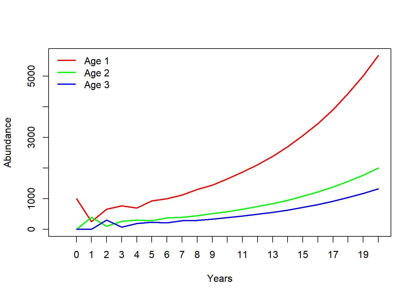
Compute lambda
Clearly this is a growing population. But let’s see exactly what \(\lambda\) is!
NOTE: we are using a “package” in R to make these analyses super easy! So if you don’t already have the “popbio” package, go to the “Packages” tab in Rstudio (should be at the top of the lower right panel), click on “Install”, and then type “popbio” in the “Packages” field in the pop-up window, then click on the “Install” button.
# Use 'popbio' package to compute lambda and SSD -----------

# Use the following line of code if you haven't installed 'popbio' yet. Once you've installed it, you can delete the line or comment this line out by adding a pound sign before the "i" in "install.packages"

# install.packages("popbio")   # uncomment this line to run - you only need to do this once

# Use the 'popbio' package to compute lambda (NOTE: you first have to install the popbio package! You only have to install the package once...)

library(popbio)   # load the 'popbio' package in R

lambda(pop_matrix)
## [1] 1.13162Pretty easy!
Compute stable stage distribution (S.S.D.)
Clearly the population doesn’t reach a stable stage distribution until a few years into our simulation. What exactly is the stable stage distribution here? We can do this in R:
# Use the 'popbio' package to compute the stable stage distribution!

stable.stage(pop_matrix)
## [1] 0.6298233 0.2226270 0.1475497This gives us the fraction of the population that is in each stage at the stable stage distribution. For example, 63% of this population will be age-1 individuals at the stable stage distribution. This vector will always sum to 1, since all the pie slices must equal the whole pie.
Note: if I gave you an initial abundance (e.g., 1000) and asked you to initialize the population at stable stage distribution, just multiply the initial abundance by this vector. For example, 1000*0.63 = 630 age-1 individuals at time 0.
Let’s get started with running some matrix-based population models!
Exercise 1: age-structured (Leslie) matrix projection models!
In this exercise, you will have a chance to play around with an age-structured (Leslie) matrix population model. But first, you are asked to translate a life table into an age-structured transition matrix!
Here is the life table: Excel
format
CSV format
| x | S(x) | b(x) |
|---|---|---|
| 0 | 1000 | 0.0 |
| 1 | 212 | 0.0 |
| 2 | 150 | 2.9 |
| 3 | 110 | 4.2 |
| 4 | 30 | 2.5 |
| 5 | 0 | 0.0 |
Translate the above life table into an age-structured (Leslie) transition matrix with four ages: age 1 (yearlings), age 2, age 3, and age 4. You don’t need to include age 5 because no individuals ever make it past age 4 (age 4 represents all individuals that have lived from 4 to 5 years of life- and no one makes it to age 5.
Keep the following points in mind:
- There is no “age 0” (newborn) stage (since this is a “pre-breeding
census” model). Individuals only “enter” the model if they are born and
survive to age 1.
- Individuals are in the “age 1” stage if they are between the ages of
1 and 2 (that is, they are one-year-olds!). They transition to the “age
2” stage (\(P_{1 \rightarrow 2}\)) only
if they survive to age 2.
- For individuals of the “age 1” class to contribute new offspring to
the population in the next time step (\(F_1\)), they have to produce offspring when
they are exactly 1 year of age (which they do at the rate of \(b(1)\) – the birth rate at age 1), and
their offspring must survive their first year of life (\(P_{0 \rightarrow 1}\)).
- Use four age classes for your transition matrix (age 1 through 4).
Individuals in the final age class (age 4) have zero survival (you can’t
survive to age 5) but a non-zero fecundity (four-year-olds can give
birth, and their offspring can survive to become one-year-olds next
year)
- No individual ever stays the same age - they either transition to the next age or they die (this is how a Leslie Matrix model works).
NOTE: Gotelli uses the term ‘age class 1’ to refer to individuals in their first year of life (0-year-olds) and ‘age class 2’ for individuals in their second year of life (one-year-olds), but I think it’s easier to think of this as age 0, age 1, etc. That way, our age classes will match the way we usually talk about age in years! But you will see other ways of describing age classes in the literature- we just have to get used to it eventually…
NOTE: The Gotelli book focuses on the type of matrix population model known as a “post-breeding census model”. This model is more difficult to understand (in my opinion) and more prone to mistakes than the pre-breeding census model, so I have chosen to focus on the pre-breeding census model in this course.
1a (image upload). Upload an image file of the full transition matrix (16 numbers, arranged in 4 rows and 4 columns) to WebCampus. To maximize our abililty to give you partial credit, please include all calculations you needed to arrive at your final solution.
1b (short answer). Describe (in words) how you computed the number in row 1, column 3 of your matrix (fecundity of 3-year-olds).
You will need to use R for the next few questions. Make sure you have the ‘popbio’ package installed in your R session!
You will need to enter your matrix from 1a into R, using something like the following:
# Construct a four-age matrix:

pop_matrix <- matrix(     #
  c(
    0,     2.5,   1.2,    0.5,
    0.3,     0,     0,      0,
    0,       0.8,  0,      0,
    0,       0,     0.55,   0
  )
  ,nrow=4,ncol=4,byrow=T
)
pop_matrix
## [,1] [,2] [,3] [,4]
## [1,] 0.0 2.5 1.20 0.5
## [2,] 0.3 0.0 0.00 0.0
## [3,] 0.0 0.8 0.00 0.0
## [4,] 0.0 0.0 0.55 0.01c (short answer- two numbers). First, what is the finite rate of growth (\(\lambda\)) for this population? (HINT: use the ‘lambda()’ function from the popbio package). Second, what is the intrinsic rate of growth (\(r\)) for this population, assuming continuous population growth? For the second part, recall that \(N_{t+1} = N_te^r\), implying \(\frac{N_{t+1}}{N_t} = e^r\), implying \(\lambda = e^r\), finally implying that \(ln(\lambda) = r\).
1d (short answer). Based on this result, is this a growing population (above replacement)? A declining population (below replacement)?
1e (short answer- 4 numbers). What is the stable-stage distribution (SSD) for this population (fraction of the population in each age after the simulation stabilizes)? (HINT: use the ‘stable.stage()’ function from the ‘popbio’ package) (HINT: a complete answer to this question requires exactly 4 numbers).
1f (short answer- 4 numbers). Assuming an initial population size of 1000 at stable stage distribution (SSD; see answer from 1e), how many individuals would you have in each of the four ages? (NOTE: you can’t have fractional individuals, so please round to the nearest whole numbers).
Next, use R to project this population for 30 years (you can re-use much of the code supplied above). Initialize your population with 1000 individuals at stable stage distribution (your answer from part 1f).
1g. (short answer- one number). What is the total number of 3-year-olds in the population after 30 years?
1h. (short answer- one number). What is the total population abundance (sum of abundances across all ages) after 30 years?
NOTE: for questions 1g and 1h remember that year 30 is actually the 31st column of Nmat, since the first column represents year 0.
Finally, run your simulation again, this time starting with all 1000 individuals in age 1 (initial abundance vector is 1000 one year olds, and zero for all other ages) instead of distributing them across all ages. This time, run your model for 50 years.
1i. (image upload). Upload an image (plot) of simulated abundance over time for all four ages. The x-axis should represent time in years (years 0 to 50), and the y axis should represent abundance. The plot should include 4 lines, one for each age. (HINT: you can re-use the R code above to produce this plot).
Exercise 2: translate InsightMaker to age-structured projection matrix!
Return to the InsightMaker model you created in Lab 3 (exercise 3 – that is, an age structured population model. Your model should look something like this:
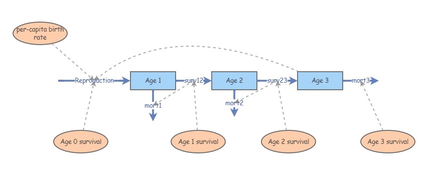
Make sure the parameters are at the original values specified in Exercise 3 of Lab 3 (before altering mortality rates as part of lab 3 question 3c). As a reminder, here they are again:
Age 3 birth rate: 12 (12 female offspring per female, assuming a
female only model)
Age 0 survival: 0.1 (10%)
Age 1 survival: 0.9 (90%)
Age 2 survival: 0.5 (50%)
Age 3 survival: 0 (100% mortality- no individuals survive to age
4)
Initial N, Age 1: 100
Initial N, Age 2: 100
Initial N, Age 3: 50
For the mortality rates, note that all individuals in the Age 1 stock must either transition to Age 2 or die. In addition, all individuals in the Age 3 stock must die- there is no Age 4 class!
Translate this InsightMaker model into a projection matrix with three rows and three columns. Pay close attention to the difference between survival (transition to the next stage class) and mortality (mortality is equal to one minus survival).
2a (image upload). Upload an image file of the full transition matrix (9 numbers, arranged in 3 rows and 3 columns) to WebCampus. To maximize your chance for partial credit, include all calculations you needed to arrive at your final solution.
Starting with 75 individuals, all in Age 1 (75 age 1, 0 age 2, 0 age 3), project this population 20 years into the future, using both InsightMaker and R.
2b (image upload). Upload an image (plot) of abundance over time for all ages, produced using R. The x-axis should represent time in years (years 0 to 20), and the y axis should represent abundance. The plot should include 3 lines, one for each age. (HINT: you can re-use the R code above to produce this plot).
2c (image upload). Upload an image (plot) of abundance over time for all ages, produced using InsightMaker. The x-axis should represent time in years (years 0 to 20), and the y axis should represent abundance. The plot should include 3 lines, one for each age.
HINT: check your answers to 2b and 2c by comparing the two plots: These plots should look essentially identical!
Now let’s build an InsightMaker model based on a population matrix!
Exercise 3: translate stage-structured projection matrix to Insightmaker!
Use the following stage matrix to answer questions 3a-b
Here is a stage-based matrix to use for building your InsightMaker model:
Click here to download the CSV
file.
Click here to download the same matrix
as an Excel file.
stmat <- read.csv("stage_matrix1.csv")
stmat <- as.matrix(stmat[,-1])
rownames(stmat) <- colnames(stmat)
stmat
## Stage1 Stage2 Stage3
## Stage1 0.1 0.65 0.90
## Stage2 0.3 0.20 0.00
## Stage3 0.0 0.35 0.75# lambda(stmat) Build an InsightMaker model that represents the same population as the stage-based matrix above. Remember that the top row represents fecundity terms, while the remaining rows represent transition terms. Also remember how to convert between survival rates and mortality rates (mortality equals one minus survival). Initialize the model with 100 individuals at stable stage distribution (SSD).
3a (short answer). Provide the URL to your InsightMaker model (and remember to clone your Insight to ensure that you don’t alter the model after you submit it).
Next, project this population 20 years into the future using both R AND InsightMaker.
3b (image upload). Upload an image (plot) of abundance over time for all ages, produced using R. The x-axis should represent time in years (years 0 to 20), and the y axis should represent abundance. The plot should include 3 lines, one for each age.
3c (image upload). Upload an image (plot) of abundance over time for all ages, produced using InsightMaker. The x-axis should represent time in years (years 0 to 20), and the y axis should represent abundance. The plot should include 3 lines, one for each age.
HINT: check your answers to 3b and 3c by comparing the two plots: These plots should look essentially identical!
NOTE: In this class we have stressed the importance of density dependence in determining and regulating the dynamics of real populations. Were any of the population models in this lab density-dependent? [Answer: NO! In adding one new type of complexity to our models- age structure- we have temporarily “forgotten” about density-dependence!]
Exercise 4. Translate written population description to projection matrix!
As a test of your understanding, build a matrix projection model based on the following written passage:
We assumed that the buff-breasted rat-hawk life history could be described in terms of four life stages: juvenile (one-year-olds), subadults (2-year-olds), non-territorial adults, and territorial adults (all individuals 3 years old and beyond are considered adults). We assumed that territorial adult females experienced an average of 12% mortality each year, and non-territorial adults experienced 25% mortality annually. Juvenile female mortality was 20% per year, and subadult mortality was 15%. Fledglings had a 30% chance of surviving their first year of life. We assumed that 90% of surviving subadults would become non-territorial adults, while the remaining 10% would become territorial adults. We assumed that 55% of surviving non-territorial females would successfully transition to the “territorial adult” stage, while 8% of surviving territorial adults would lose their territories, becoming non-territorial adults. Territorial adults are the primary reproductive stage, and produce an average of 3.4 fledged hatchlings each year, half of which are female. Non-territorial adults produce 0.6 new fledged hatchlings each year on average, half of which are female. We ran a female-only matrix population model, and we initialized the population with 800 juveniles, 150 subadults, 75 non-territorial adults and 50 territorial adults.
4a (image upload). Upload an image file of the full transition matrix (16 numbers, arranged in 4 rows and 4 columns) to WebCampus. To maximize your chance for partial credit, include all calculations you needed to arrive at your final solution.
4b (short answer: four numbers). How many juveniles, subadults, non-territorial adults and territorial adults would there be in the population at time 0 if you were to initialize the population with 1000 individuals at S.S.D.? (1000 total individuals at time 0).
4c (one number). What is the finite growth rate, Lambda, for this population?
##Checklist for Lab 4 completion
Please submit all responses using WebCampus!
As always, URLs for your InsightMaker models should be pasted in your lab submission (in WebCampus). See details below…
see WebCampus for submission deadline
- Webcampus submission
- Exercise 1
- image upload (1a.)
- short answer (1b.)
- short answer (1c.)
- short answer (1d.)
- short answer (1e.)
- short answer (1f.)
- short answer (1g.)
- short answer (1h.)
- image upload (1i.)
- image upload (1a.)
- Exercise 2
- image upload (2a.)
- image upload (2b.)
- image upload (2c.)
- Exercise 3
- short answer (3a.)
- image upload (3b.)
- image upload (3c.)
- Exercise 4
- image upload (4a.)
- short answer (4b.)
- short answer (4c.)
- Exercise 1
—End of Lab 4—-