Population regulation
NRES 470/670
Spring 2026
What is density dependence (D-D)?
As part of Lab 1 we went through the mathematics of exponential growth. This week we will explore basic models of density dependence. Exponential growth, as you have seen, leads to a runaway ‘snowball effect’. It is not sustainable. As Malthus noted, resources are finite, and sooner or later exponentially growing populations will find their limits.
Density: In D-D, density refers to the number of conspecifics that you are competing with for food and/or other resources. The more you compete with others of your own species, the less favorable your vital rates become (e.g., per-capita death rate, d, increases or per-capita birth rate, b, decreases)! As N goes up, vital rates take a turn for the worse.
If vital rates become less favorable to growth as population density increases, this is known as negative density dependence (as abundance goes up, the per capita growth rate does down!). This is a kind of negative feedback.
Regulation!
First of all, we have already established that positive feedbacks are not sustainable: increases in some stock lead to faster increases, leading to faster increases, etc. (i.e., the vicious circle of exponential growth). Density dependence is also a feedback, but it is a negative feedback! Which is also known as a stabilizing feedback. As we discussed before, negative feedbacks are essential for regulated systems. Recall the example of homeostasis in organismal biology. If blood sugar goes up, the body will work to lower it, and vice versa.
Same with populations. In a regulated population, an increase in abundance will cause a decrease in the population growth rate, and a decrease in abundance will cause an increase in the population growth rate (compensatory growth).
You can’t have a self-regulated system without some kind of negative feedback.
Q: Is density-dependent population regulation a “law of nature”?
Logistic growth
Logistic growth can be described mathematically by the following equation:
\[\Delta N = r_{max} N_t \left ( 1 - \frac{N}{K} \right )\]
This is the second most important equation of population ecology (after basic exponential growth!).
We will go into more detail in lab, but let’s break this equation down a bit.
The first part of this equation looks familiar, right?
\[\Delta N = r \cdot N_t\]
What about the second part,
\[\left ( 1 - \frac{N}{K} \right )\]
You can think about \(\frac{N}{K}\) as the used portion of carrying capacity
By the same token, you can think about \(\left ( 1 - \frac{N}{K} \right )\) as the unused portion of carrying capacity (or the relative ‘un-crowded-ness’ of the habitat).
When carrying capacity is mostly unused, population growth resembles exponential growth!
When carrying capacity is mostly used up, population growth resembles, well…, no growth at all!
Q: Given the two above statements, can you figure out what population dynamics (that is, abundance vs. time) should look like under logistic growth, starting with a very small population?
Carrying capacity is an equilibrium!
A stock-flow system is at equilibrium when [Flows In] are equal to [Flows Out]. That is, if opposing forces cancel each other out.
As Gotelli shows, and we will go over in detail in lab 2, you can derive the logistic growth equation by making b and d (from the standard population growth equation) both linear functions of population size (density) \(N\):
\[b=b_{max}-aN\]
where \(b_{max}\) is the maximum, or ideal, per-capita birth rate and \(a\) is the density dependence term (amount by which birth rate declines with each new individual added to the population).
Similarly,
\[d=d_{min}+cN\]
where \(d_{min}\) is the minimum (most favorable) per-capita death rate (1-maximum survival rate) and \(c\) is the density dependence term (amount by which death rate increases with each new individual added to the population).
We can plot these equations out in R:
Density <- seq(0,500,1)  # create a sequence of numbers from 0 to 500, representing a range of population densities

## CONSTANTS

b_max <- 0.8  # maximum reproduction (at low densities)
d_min <- 0.3  # minimum mortality

a <- 0.001    # D-D terms
c <- 0.0005

b <- b_max - a*Density
d <- d_min + c*Density

plot(Density,b,type="l",col="green",lwd=2,ylim=c(0,1),main="Density-Dependence!",ylab="b or d")
lines(Density,d,col="red",lwd=2)
axis(4,at=seq(0,1,0.2))
#mtext("d",4)
legend("bottomleft",col=c("green","red"),lty=c(1,1),legend=c("per-capita birth rate","per-capita mortality"),bty="n")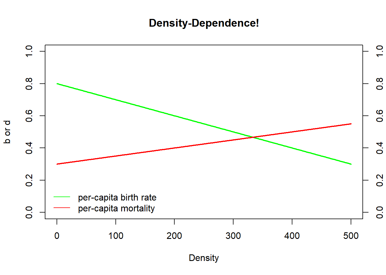
What is the equilibrium point in this system? That is, what is the (non-zero) abundance/density at which population growth is equal to zero??
This equilibrium is known as K, or carrying capacity?
Equilibria can be stable or unstable (see below). This distinction is critical for wildlife managers and conservation biologists to understand.
Stable and non-stable equilibria
First, when we add or subtract a small number of individuals to a population that is at an equilibrium, we say we have ‘perturbed’ the system.
A stable equilibrium, when perturbed, returns to the equilibrium point
A non-stable equilibrium, when perturbed, does NOT return to the equilibrium point
Is the image on the left a stable or a non-stable equilibrium??
What about the image on the right?
What about K, or carrying capacity?
Let’s find out!
In-class exercise: logistic growth
First of all, remember to save your working InsightMaker models, since we will often be building from previous models (so we don’t have to start from scratch every class!).
To build off of a previous Insight, open a previous Insight (e.g., your basic exponential growth model– or clone this model) and choose “Clone Insight” in the upper right corner to create a copy that you can edit.
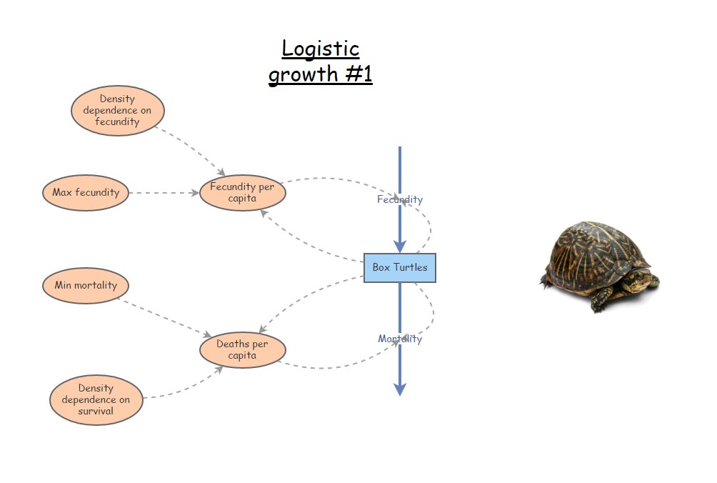
Here is the scenario we will model: both b and d are density-dependent. We will replicate the model from the R code and figure above- this time in InsightMaker!
CONSTANTS
- [Maximum per-capita birth rate] = 0.8 individuals per individual per year
- [Minimum per-capita death rate] = 0.3 individuals per individual per year
- [Density dependence on fecundity] (a) = 0.001
- [Density dependence on mortality] (c) = 0.0005
EQUATIONS
- [Per-capita birth rate] = [Maximum per-capita birth rate] - [Density dependence on fecundity] * [Abundance]
- [Per-capita death rate] = [Minimum per-capita death rate] - [Density dependence on mortality] * [Abundance] How can we do this in InsightMaker?
Load a basic exponential growth model. Rename the main [Stock] Turtles (or your favorite animal!). This [Stock] should have two [Flows], one [Flow In] named Births and one [Flow Out] named Deaths. Both Births and Deaths should be defined as the product of Turtles and per-capita rates, respectively called Births per capita and Deaths per capita (each defined on the canvas as [Variables]). This model should be very familiar by now!!
Initialize the population to 5 (way below carrying capacity).
Make four new [Variables] on the canvas, to represent the four key rates in our model (max. birth rate, dropoff in birth rate with each new individual added to the population, min. death rate, slope of death rate with increasing abundance).
Set the Maximum per-capita birth rate to 0.8 (turtles produced per turtle per year). Set the Minimum per-capita Death rate to 0.3. Set the Density dependence on fecundity to 0.001. Set the Density dependence on mortality to 0.0005.
Make the appropriate connections, as in the figure above, and use the equation window to make sure the equations are correct.
Change the settings so that the simulation runs for 100 years.
Your model should look something like this!
For the purpose of answering the questions below, here is a functioning model you can use as a starting point:
- Run this model. Does the model behave as you would expect?
Q: What is carrying capacity in this model?
Q: What happens if population size starts out
at carrying capacity? [Top Hat]
Q: What happens if population size starts out
above carrying capacity? [Top Hat]
Q: Is carrying capacity (K) a stable equilibrium in
this model? [Top Hat]
Q: In real-world systems, is carrying capacity stable? Is it an equilibrium point?
- Consider the basic logistic growth equation:
\(\Delta N = r_{max} \cdot N_t \cdot \left ( 1 - \frac{N}{K} \right )\)
Q: What happens if \(r_{max}\) is zero? What happens to carrying
capacity?
Q: Which population is more likely to be found at or
near K in nature? A population with very large \(r_{max}\) or very small \(r_{max}\)?