Grizzly bear PVA example
NRES 421/621
Spring 2024
In this module we will use a PVA to do investigate the future of the grizzly bear population in Yellowstone National Park.
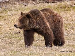
Our goal is to better understand the conservation outlook for the grizzly bear population in Yellowstone park, and how many bears the park may be able to support!
But first, let’s look at the process of building a PVA model:
A general PVA workflow
Step 0: Define your questions/hypotheses!
Like any scientific research, you first need to start with one or more testable research questions. For PVA, this might be:
- What is the extinction risk for a focal population over a specific time horizon (e.g., 100 years)?
- What is the minimum viable population size for my focal population?
- Of the conservation actions currently being proposed for my focal species, which is likely to have the greatest bang for the buck?
- Many more!
Once you have your research questions, the basic process looks something like this:
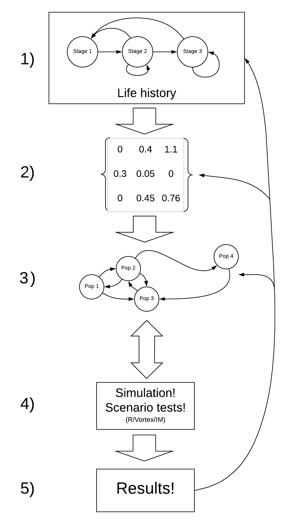
Step 1: Life history
How does your population work?
The first step (after you have formulated your research questions, of course!) is to conceptualize the life history of your focal species. In general, the following life history traits are often critical to consider:
- Maximum and minimum reproductive age
- Number of relevant age classes
- Density-dependence mechanisms
- Which vital rates may be sensitive to environmental conditions (e.g., annual rainfall)?
- And more…
Step 2: Parameterize the demographic model!
This is where you attach numbers to the stocks and flows in your conceptual life history diagram!
These numbers include survival rates, birth rates, density-dependence terms, year-to-year environmental variability, initial abundance, and more.
Step 3: Spatial structure (metapopulations)!
If you want to ask spatial questions, your model needs to be spatially explicit. The kinds of questions you might think about include:
- How many discrete subpopulations in your focal landscape?
- At what rate do individuals move/disperse among these populations?
For the grizzly bear and loggerhead examples, we will not consider spatial structure!
Step 4: Simulate under alternative scenarios!
There are lots of options for simulation software- R, InsightMaker, Vortex, Ramas, and much more!
The key question here is: what scenarios do you want to test in order to answer your original research questions?
Step 5: Results
Finally, you need to make sense of all the simulations you just ran!
There are two major tools that you will need to do this: graphical visualization and statistical analysis.
NOTE: The process of building a PVA model is iterative and non-linear.
For example – after running your model (step 4) you might realize that your results (step 5) are unrealistic. This might prompt you to go back to the literature and change your parameter estimates to something more realistic (step 2).
PVA for Yellowstone grizzly bears!
Okay, now let’s build a PVA model together- this time focusing on the Yellowstone grizzly bear population!
Step 1: conceptualize the life history
Based on a literature review, we determined that there are four main stages in the grizzly bear life history: cub, yearling, subadult and adult! The adult stage is the only one that is reproductive! Furthermore, the subadult stage lasts approximately 3 years, from the 3rd to the 5th year of life.
Therefore, our conceptual life history diagram looks something like this!
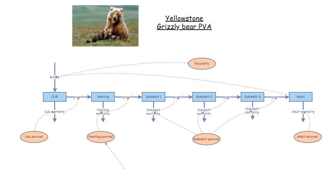
You can “clone” the base grizzly bear model here. This model has not yet been parameterized!
Step 2: parameterize the model!
Let’s use the following table to parameterize the population vital rates and initial abundances in our model!
This table actually has two alternative parameterizations, one summarized from data collected during the period from 1983 through 2001, and the other representing data from the period from 2002-2011.
NOTE: we are not paying any attention to males! Population models are often female-only, since females are usually the primary drivers of population dynamics.
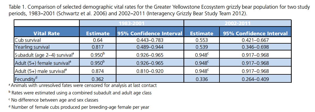
The table is from this scientific report (alternative link)
What about population size?
From Schwartz et al 2006 we know that:
- Adult (reproductive) females represent approximately half (50%) of the total female population.
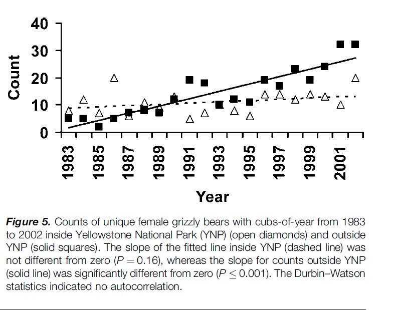
- Total abundance of adult females in the greater Yellowstone park area (solid squares plus the open triangles) was ca. 10 in 1983 and ca. 40 in 2001/2002
Let’s use the initial (1983) abundances (all female!) to initialize our model:
Cubs: 3
Yearlings: 3
Subadult 1: 2
Subadult 2: 2
Subadult 3: 2
Adults: 10
Take a few minutes to parameterize the model, using the 1983 to 2001 estimates from the table above!
Step 3: Simulate!
Okay, let’s run the model!
- Try running the model with the parameterization we discussed above. What do you notice? Is the population growing?
REALITY CHECK:
Q: Given that the population of adult females is known to have increased to around 40 by the year 2002, is this model realistic??
- What if we configure the model to run for 100 years? What happens now?
Short Answer Question: Based on the 100-year simulation, do you think this model of the Yellowstone grizzly population is biologically realistic? Why or why not?
- Now let’s change the parameterization to reflect the vital rates observed for the period 2002 to 2011 in the table:
In 2002 the population was more like 40 females- so let’s use the following values for the initial population size!
Cubs: 15
Yearlings: 15
Subadult 1: 5
Subadult 2: 5
Subadult 3: 5
Adults: 40
Q: What do you notice about this model? Is the population still growing? What about the overall rate of growth of the population?
Short Answer Question: Which vital rates changed the most from 1983 to 2002? Can you think of any reason for this change?
Density-dependence
- Let’s implement a new process into our model- density-dependence!
We know that when the total (female) population size was around 20, yearling survival was around 82%
We also know that when the total (female) population size was around 80, yearling survival dropped to around 54%
What is the linear relationship between population size and yearling survival? When abundance increased by 60, yearling survival rate decreased from 82% to 54% – a 28% drop!
SLOPE: For each additional individual in the adult population, yearling survival decreased by 0.47% (\(=\frac{0.28}{60}\)).
INTERCEPT: This can be interpreted as the expected yearling survival when there are no adults in the population. When there were 10 female adults, yearling survival was 81.7%. If there were 0 individuals in the adult population, yearling survival would (theoretically) be \(81.7 + 0.47\cdot 10\), which is 86.4%.
So the linear formula for computing yearling survival as a function of adult female abundance should be:
\(Surv_{yearling} = \frac{\left ( 86.4 - 0.47*N_{female} \right )}{100}\)
NOTE: we divide by 100 to convert the result from a percentage to a fraction
Let’s implement this density-dependent process in Insightmaker!
Use your existing model or load and clone this InsightMaker model.
Open the equation editor for yearling survival, and input the equation above! Let’s do it together!
Run the model! What do you notice?
Try running the model for 100 years.
What happens??
Grizzly bear in-class exercises
Working in groups is encouraged!!
To start off, you can clone a full, density-dependent version of the grizzly model here
Make sure the initial abundances are set at the estimated values for 1983 to 2001, and the model is set to run for 100 years.
Short Answer Question: What is the approximate carrying capacity (K) of the Yellowstone grizzly population? NOTE: this is an emergent property of our new, density-dependent model! We didn’t specify carrying capacity, but it emerges out of the model.“Comment out” the density dependence equation in the equation editor for yearling survival (place a pound sign before the equation; see below for more explanation). Instead, use the yearling survival estimate for the 2002-2011 time period (survival is 0.539). The “commenting out” trick enables you to easily run the grizzly bear PVA with and without the density-dependence process (using the pound signs to alternately comment out the density-dependence equation or the value ‘0.539’; see below).
Short Answer Question #4 In each case (with density-dependence and without density-dependence), what can we say about the final population abundance after 100 years?? (hint: use the ‘Sensitivity Testing’ tool; see below for more details)
Before answering the next question, comment out the density-dependence equation and set yearling survival to its lowest possible value from Table 1 (above; 0.346). This is an example of a worst-case scenario
Short Answer Question #5 Local managers have decided that a viable grizzly bear population should have no more than a 5% risk of falling below 30 total individuals at any time over the next 100 years, can you identify an approximate minimum viable population size (MVP) for this population under the worst-case scenario above? That is, try to find a set of initial abundances (initial abundance for each of the six age-classes) such that you can’t reduce the population any further without having an unacceptable (>5%) risk of falling below 30 individuals over the next 100 years.
Helpful hints to answer the grizzly bear questions
“commenting out” the density-dependence equation
You can turn the density dependence process on and off by using the pound symbol to “comment out” the equation. So … if you input the following into the equation editor for yearling survival, you can easily go back and forth between the density-dependent and the density-independent formulations of the model:
For example, this one is density-independent:
0.539
#0.864-0.004666*[Total abundance]
…and this one is density-dependent:
#0.539
0.864-0.004666*[Total abundance]
…or for the worst case scenario:
#0.539
#0.864-0.004666*[Total abundance]
0.346
using the sensitivity testing tool to evaluate risk
Use the “sensitivity testing” option in the “Tools” menu to run multiple simulations. You can visually assess the risk of falling below a certain abundance threshold by examining whether a particular quantile (e.g., 90%) of your simulation results (the output from the sensitivity testing tool) falls below a particular threshold (e.g., 1 individuals) over a specified number of years (e.g., 50 year). For example, the following figure illustrates a population with an extinction risk of approximately 5% (90% of the simulations fall within the blue region, so 5% of simulations fell below the threshold and the remaining 5% of of simulations were larger than the upper bound of the blue region) :

You can compute the risk of extinction or decline more quantitatively as the fraction of replicates that failed to meet the specified criterion. That is, you can divide the total number of simulations falling below the threshold by the total number of replicates.